NirsBlockAverageGLMOffline

fNIRS Block Averages and GLM Analyses (Offline)

This example pipeline analyzes a single fNIRS recording (or a folder of them). It imports raw NIRS data, preprocesses it, renames the task events, and then runs two common fNIRS analyses side by side:

• Block averages: the hemodynamic response averaged across all repetitions (trials) of each condition, along with its standard error.
• General Linear Model (GLM): a regression of each channel's signal onto a canonical hemodynamic response function (HRF), giving one beta weight (and p-value) per channel and condition.

A subset of the results are plotted and also saved to a .pkl file. You can load this file in a group-level analysis pipeline, or in a third party software for further statistics and figure generation.

The example data set (NIRSMotorImagery.nirs) was recorded with a NIRx NIRSport2 headset during a motor imagery task, where the participant imagined tapping with the left or right hand. The pipeline compares left-hand and right-hand tapping for both oxygenated (HbO) and deoxygenated (HbR) hemoglobin. This example pipeline only examines the 10 second duration trials.

Before getting started, make sure that you are using Pipeline Designer with "Show expert parameters" checked (under File->Settings).

The main loop of the pipeline is shown below:

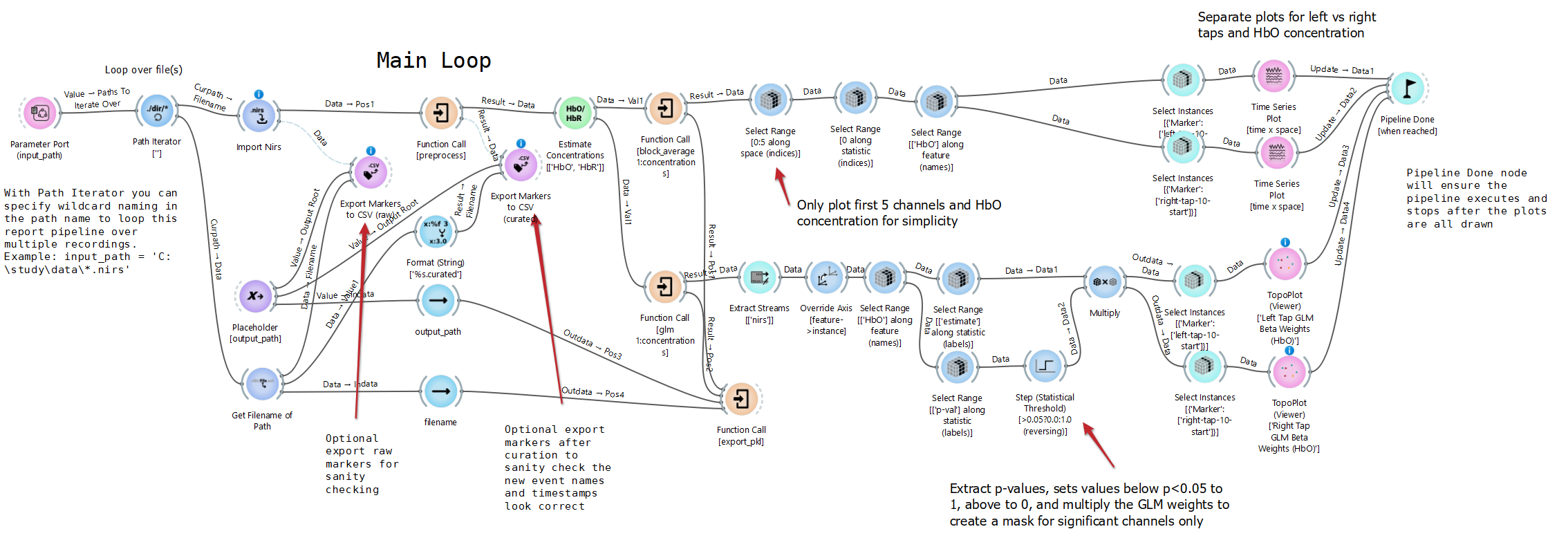
The pipeline is organized with functions. The Main Loop at the top runs once per file. It calls a series of Function Definition subgraphs that are laid out below it on the canvas: preprocess, marker_curation, block_average, glm, and export_pkl. A Global Variables section on the left holds the settings you are most likely to change. The functions can read these settings by name.

This walkthrough covers the pipeline in the following stages: global variables, data import and the main loop, preprocessing, marker curation, block averages, GLM, visualization, and export.

Global Variables

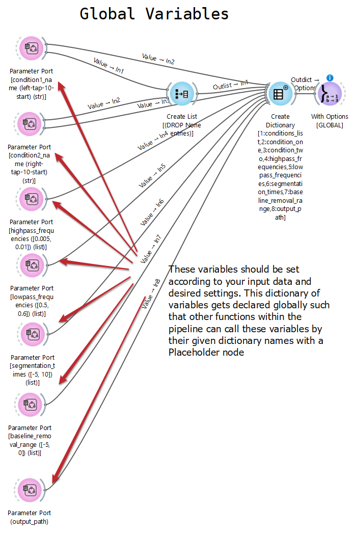
The pink Parameter Port nodes on the left are the main settings of the pipeline. When the pipeline is run from the command line or on Neuroscale, these appear as named parameters that you can override without opening the pipeline. In Pipeline Designer, double-click a node to edit its default value.

Parameter	Default	Meaning
condition1_name	left-tap-10-start	Marker name of the first condition
condition2_name	right-tap-10-start	Marker name of the second condition
highpass_frequencies	[0.005, 0.01]	High-pass rolloff and cutoff frequencies (Hz)
lowpass_frequencies	[0.5, 0.6]	Low-pass cutoff and rolloff frequencies (Hz)
segmentation_times	[-5, 10]	Window (s) cut around each event for the block average
baseline_removal_range	[-5, 0]	Window (s) whose mean is subtracted from each block
output_path	~/.neuropype/outputs	Directory to export data outputs

The two condition names are collected into a list by the Create List node. That list, together with all the other values, is packed into a dictionary by Create Dictionary. The dictionary is then passed to the With Options node with GLOBAL checked, which makes every entry available to the whole pipeline. Inside any function, a Placeholder node whose slotname matches a dictionary key (for example highpass_frequencies or conditions_list) receives that value. You can therefore change a setting in one place, and every function that uses it picks up the change.

The condition names must match the marker names in your data. With the Import Nirs settings described below, each stimulus produces a <name>-<duration>-start marker and a matching -end marker, which is where names such as left-tap-10-start come from. If you are unsure what your markers are called, see the optional marker export described in the next section.

Data Import and the Main Loop

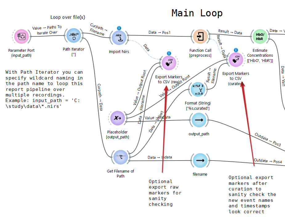
The input_path Parameter Port gives the file to analyze (the default filename provided automatically directs to where the example dataset is installed). It feeds a Path Iterator node, which runs the rest of the pipeline once for each file that matches the path. You can use wildcards to process many recordings in one run, for example input_path = 'C:\study\data\*.nirs'. The current path is also sent to Get Filename of Path node, which is used to name the output files that will be exported.

The data is loaded by the Import Nirs node. Its key settings are:

• device: nirsport2, the headset that recorded the example data.
• stim_conditions: {'1': ['left-tap', 10], '2': ['right-tap', 10]}. A .nirs file stores stimuli as columns of a stim matrix (of integer values) rather than as named string events. This setting maps values 1 to a 10-second left-tap trial and values 2 to a 10-second right-tap trial. For each stimulus, NeuroPype will segment around each matching stimulus start event marker.

Two Export Markers to CSV nodes are included for checking that the markers look right. One exports the raw markers (<filename>.markers.csv) and the other exports them after preprocessing and curation (<filename>.curated.markers.csv). Their data links are disabled by default (drawn as dashed lines). To turn on an export, right-click the dashed link and enable it.

The imported data is passed to Function Call [preprocess] and then to Estimate Concentrations node. That node converts optical density to changes in HbO and HbR concentration using the modified Beer-Lambert law, with dpf=6.0 (differential pathlength factor) and pvc=60.0 (partial volume correction). The concentration data is then sent to both Function Call [block_average] and Function Call [glm].

Preprocessing

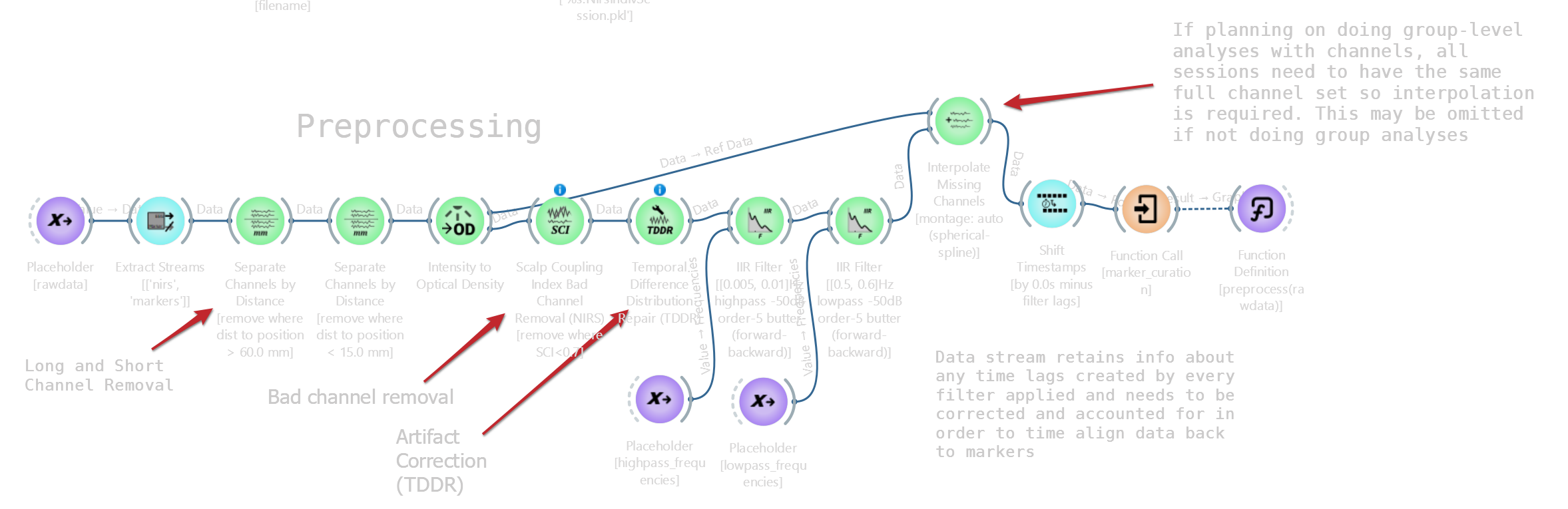
The preprocess(rawdata) function contains a standard fNIRS cleaning chain:

1. Extract Streams keeps the nirs and markers streams and drops any other streams in the file, such as accelerometer data.
2. Separate Channels by Distance (two nodes) removes channels whose source-detector distance is greater than 60 mm, and then those shorter than 15 mm. Very long channels have too little signal. Very short channels mostly measure the scalp rather than the brain. In the example file this step removes 16 short-separation channels.
3. Intensity to Optical Density converts the raw light intensities to optical density (OD), which is the form the later steps expect.
4. Scalp Coupling Index Bad Channel Removal (NIRS) removes channels with poor optode-to-scalp contact. This node first applies a band-pass filter (FIR) to avoid systematic factors such as cardiac and Mayer waves. It then checks the correlation between channels. Channels with an SCI below threshold=0.7 are removed.
5. Temporal Difference Distribution Repair (TDDR) corrects motion artifacts (spikes and baseline shifts) without needing any manually tuned thresholds.
6. IIR Filter (high-pass) removes slow drifts. The node uses a 5th-order Butterworth filter, applied forward and backward. Its frequencies input is connected to the highpass_frequencies placeholder.
7. IIR Filter (low-pass) removes cardiac and respiratory oscillations. Its frequencies input is connected to the lowpass_frequencies placeholder.
8. Interpolate Missing Channels rebuilds the channels that the scalp coupling check removed. It uses the optical density data from before that check as a reference for the full channel set (ref_data input). Long and short channels that were dropped by distance are not restored. Every session then has the same channels, which a group-level analysis needs. If you only analyze single sessions, you can bypass this node.
9. Shift Timestamps with compensate_filter_lag checked corrects for any delay the filters added to the data, so that the data lines up with the markers again.

The cleaned data is then passed to the marker_curation function before it is returned.

Marker Curation

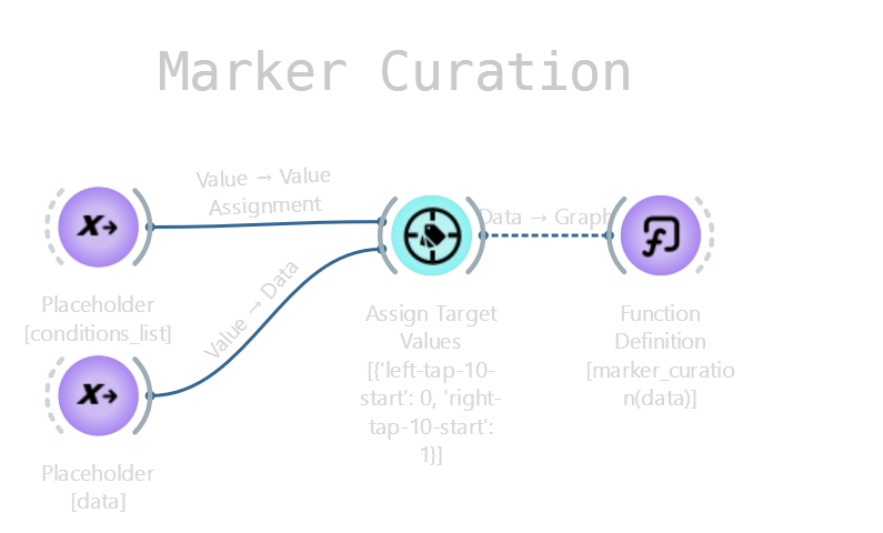
The marker_curation(data) function uses an Assign Target Values node to give each condition a numeric target value. It takes the conditions_list from the global variables, so left-tap-10-start is assigned target value 0 and right-tap-10-start is assigned target value 1. This step is necessary for Event Related Potential (Meta) node, which uses Segmentation node to create discrete trials segments. All other markers, such as the -end markers, are not given a target and are ignored by the analyses that follow.

This function is the place to add any other marker editing your data needs, such as renaming, merging, or inserting events.

Compute Block Averages

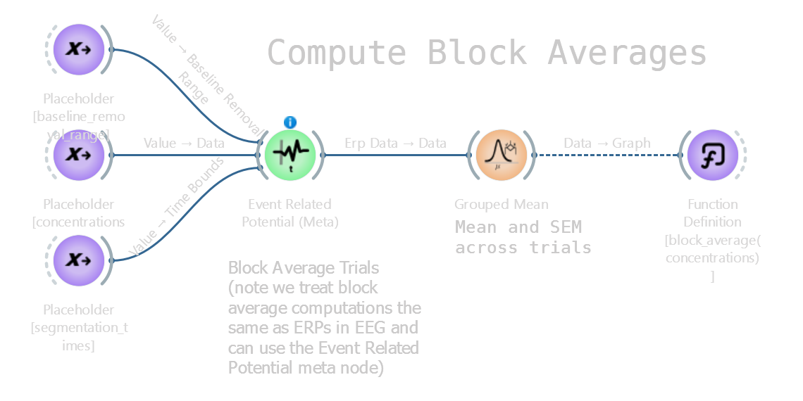
In fNIRS, a block average is computed the same way as an event-related potential (ERP) in EEG. The block_average(concentrations) function therefore uses the Event Related Potential (Meta) node:

• time_bounds (from segmentation_times) cuts a segment from 5 s before to 10 s after the start of each trial. The start/onset of each trial corresponds to the timestamps of the events that were previously assigned target values in the marker_curation(data) function.
• baseline_removal_range (from the global variable of the same name) subtracts the mean of the 5 s before each block. The responses then show the change from rest.
• output_measure is set to trials, so the node returns every segment instead of averaging them.

The Grouped Mean node then averages the segments separately for each Marker value (group_cols=['Marker']). It outputs the mean and the standard error of the mean (error_type='sem'), one instance axis element per condition.

Compute GLM

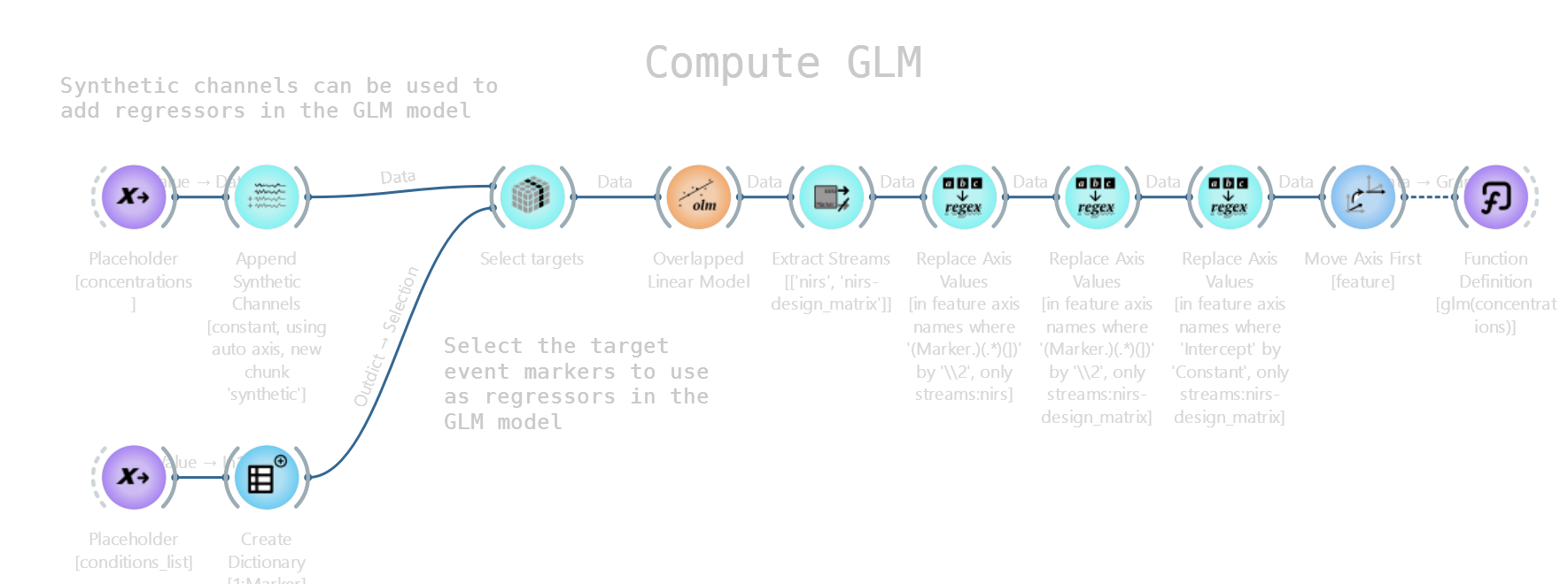
The glm(concentrations) function fits a GLM to the continuous (unsegmented) concentration data:

1. Append Synthetic Channels adds a synthetic stream containing a constant regressor, which acts as the model's intercept. You can add other nuisance regressors here, such as linear trends or DCT drift terms, by changing family.
2. Select targets keeps only the markers named in conditions_list. The Create Dictionary [1:Marker] node builds the selection {'Marker': conditions_list} from the global variable. This setting overrides the default selection stored in the node.
3. Overlapped Linear Model fits the model to the nirs stream. With response_model='canonical hrf', each condition is modeled as a canonical hemodynamic response that covers the onset and duration of each block. robust estimation (Tukey bisquare IRLS) reduces the influence of outliers. max_autocorr_delay=4.0 fits an autoregressive noise model alongside the response model, which accounts for the strong serial correlation in fNIRS noise. The output holds one estimate (beta), p-val, and related statistics per channel, chromophore, and condition.
4. Extract Streams, three Replace Axis Values nodes, and Move Axis First tidy up the result. They change regressor names such as Marker[left-tap-10-start] to just left-tap-10-start, rename Intercept to Constant, and move the regressor (feature) axis to the front.

Visualization

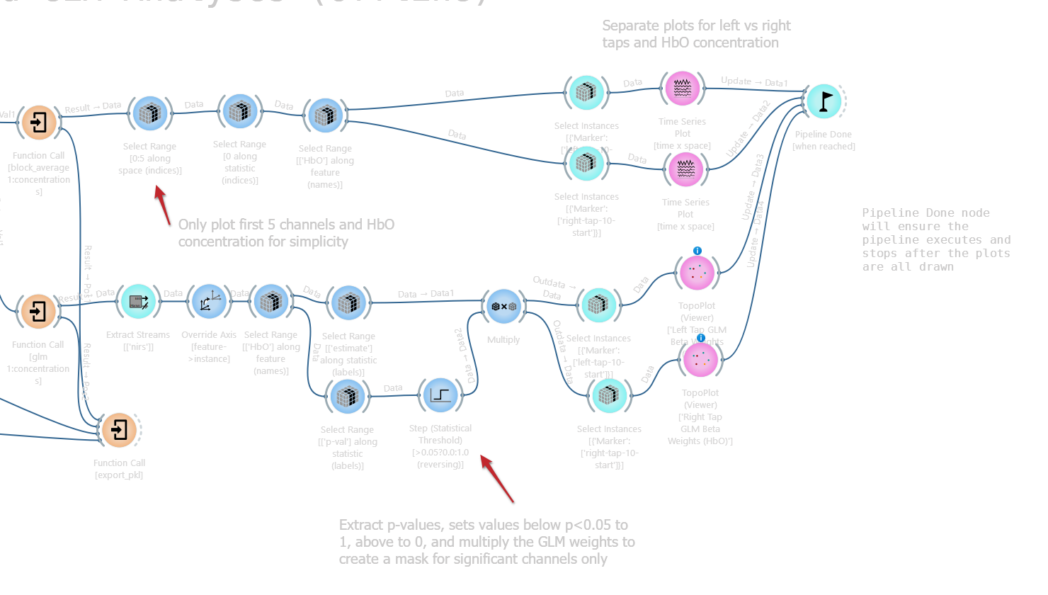
Back in the main loop, the results are plotted. For simplicity, each plot shows only HbO and the first 5 channels.

Block averages: Select Range nodes keep channels 0:5 along the space axis, the mean statistic (index 0), and the HbO chromophore. A pair of Select Instances nodes then splits out the left-tap and right-tap conditions, each feeding a Time Series Plot node:

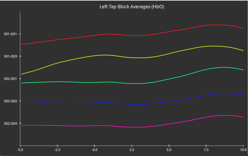
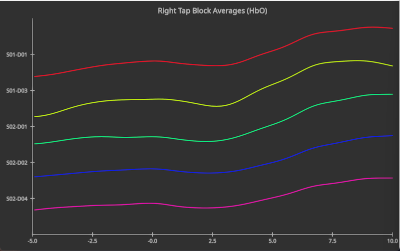
The x axis is time in seconds relative to the start of the block, from -5 to 10 s. A typical hemodynamic response shows HbO rising a few seconds after the block starts.

GLM beta weights: The GLM output goes through Override Axis node (feature to instance), so that the conditions can be selected with Select Instances node. It then goes through Select Range node to keep HbO concentration only. Next, the estimate and the p-val statistics are taken out on separate branches. The p-values go into a Step node with threshold=0.05, which turns them into a mask: 1 where p < 0.05 and 0 otherwise. Multiply node applies this mask to the betas, so only significant channels keep a non-zero value. Finally, the left-tap and right-tap results are drawn in TopoPlot (Viewer) nodes, which show each channel as a line between its source and detector on the head:

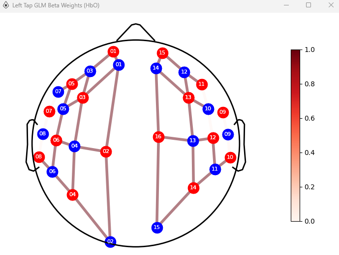
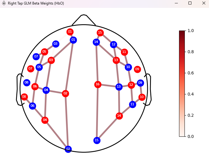
Motor imagery is expected to activate the motor cortex. To check this, compare the maps and look for significant HbO beta weights over the central motor cortex.

All four plots are connected to a Pipeline Done node, which stops the pipeline once every plot has been drawn. Otherwise this offline pipeline would keep running.

Export for Group Analysis

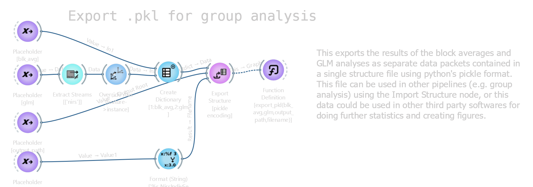
The export_pkl(blk_avg, glm, output_path, filename) function saves both results to one file. The GLM result is reduced to the nirs stream and its feature axis is changed to an instance axis. Then Create Dictionary combines it with the block averages into {'blk_avg': ..., 'glm': ...}. Export Structure writes this dictionary in Python pickle format to <filename>.NirsIndivSession.pkl, in the same folder as the input file.

You can load this file into a group-level pipeline with the Import Structure node, or in Python with pickle.load to run further statistics or make figures in other software.

Running the Pipeline on Your Own Data

1. Set input_path to your file, or use a wildcard such as C:\study\data\*.nirs to process several files.
2. In Import Nirs, set device to your headset. Set stim_conditions to match the columns, names, and durations of your stim matrix.
3. Turn on the curated marker export (see above), run the pipeline once, and check the marker names in <filename>.curated.markers.csv.
4. Set condition1_name and condition2_name to the -start markers of your conditions.
5. Adjust the filter bands, segmentation_times, and baseline_removal_range to suit your block length and design.
6. Update the condition names in the plotting Select Instances nodes and the plot titles in the main loop. These are set directly on the nodes, not taken from the global variables.

Outputs written next to each input file:

• <filename>.markers.csv: raw markers with timestamps (when enabled)
• <filename>.curated.markers.csv: markers after curation (when enabled)
• <filename>.NirsIndivSession.pkl: block averages and GLM results for group analysis