Alpha peak frequency and amplitude

This example pipeline, AlphaPeakFrequencyAmplitude.pyp, computes the spectrum of an EEG stream in real time and extracts two numbers from a chosen frequency band: the peak frequency (the frequency, in Hz, at which power is highest) and the peak amplitude (the power at that peak, in dB). By default the band is alpha (8-13 Hz), but it can be changed to delta, theta, beta or gamma with a single parameter. The results are shown live on a spectrum plot and on two bar plots, and can optionally be recorded to CSV files.

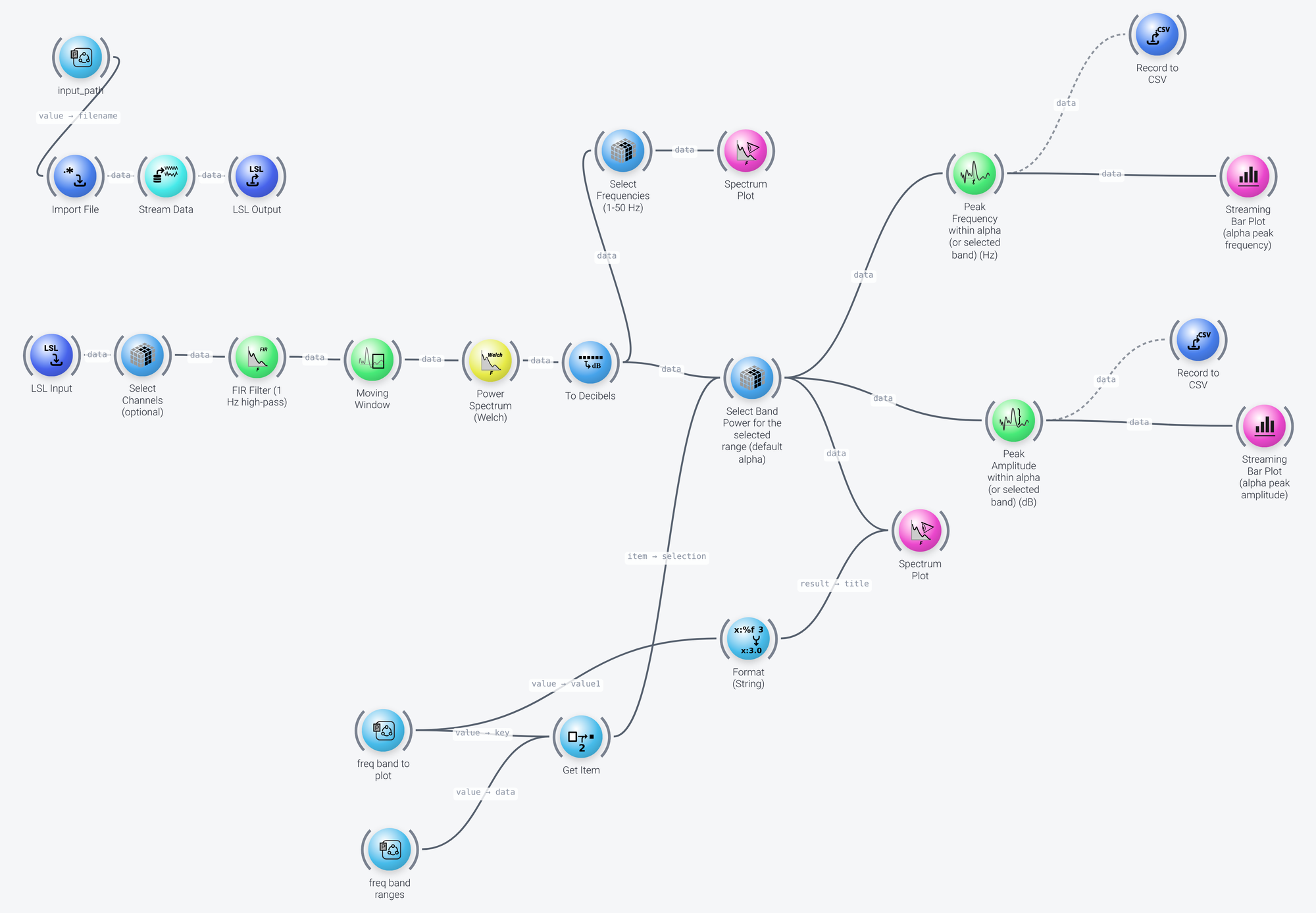
The pipeline can be divided into five parts, which we discuss in the following: data acquisition, spectral analysis, band selection, peak extraction, and output.

Data Acquisition

Includes: LSL Input, and (for the example only) Import File, Stream Data and LSL Output

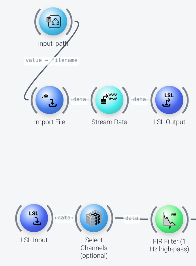
This pipeline is designed to run out of the box by restreaming recorded data. For use with live data, you would remove the playback branch and change the query property of the LSL Input node so that it finds your live EEG stream, for instance type='EEG', or the name of your device's LSL stream. For use with recorded data, change the Import File path, wire it directly into Dejitter Timestamps and drop the LSL and Stream Data nodes. See Data input in the example pipelines for details.

Spectral Analysis

Includes: Select Channels, FIR Filter, Moving Window, Power Spectrum (Welch) and To Decibels

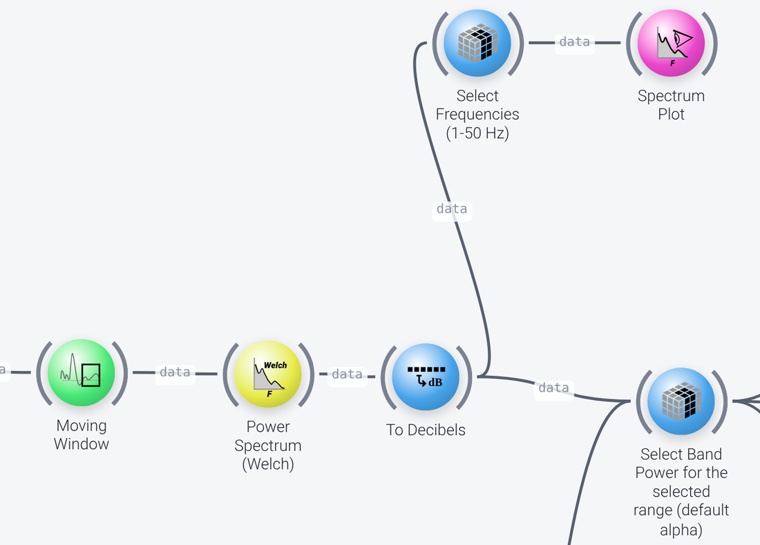
The Select Channels node (a Select Range node working on the space axis) is optional. Here its selection property keeps all but the last 6 channels (:-6), which for the example recording are non-EEG channels. Adjust or remove it to match your headset.

The FIR Filter is set up as a 1 Hz high-pass filter, which removes slow drifts that would otherwise dominate the low end of the spectrum.

A spectrum cannot be computed from continuous data directly, so the Moving Window node first cuts the stream into overlapping windows. The length of these windows is set with its window_length property, which is 2 seconds here. A longer window gives a finer frequency resolution and a smoother estimate, but the display reacts more slowly to changes. The Power Spectrum (Welch) node then computes the power spectral density for each window; see that node's documentation for how the window length affects the calculation.

Finally, To Decibels converts the power values to dB. If you would rather work with raw power spectral density values, you can remove this node.

The resulting spectrum is also displayed in the upper branch of the pipeline: a Select Range node (Select Frequencies) keeps the 1-50 Hz range (selection set to 1...50 on the frequency axis) and passes it to a Spectrum Plot.

Band Selection

Includes: Select Range, Get Item, Format (String) and the freq band ranges and freq band to plot parameter ports

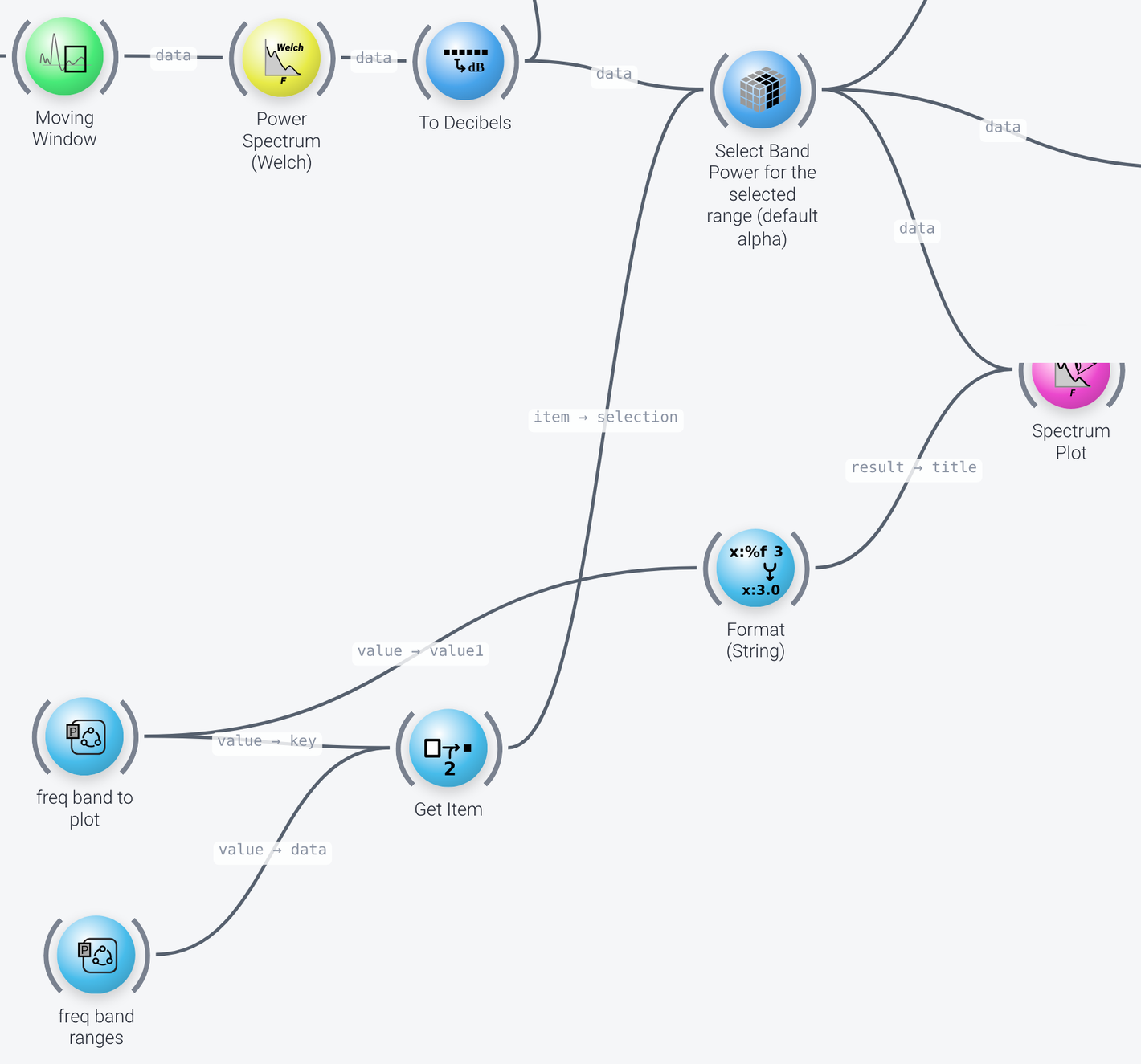
In the main branch, a second Select Range node (Select Band Power) restricts the spectrum to the frequency band of interest. It also works on the frequency axis, but its selection property is not typed in directly. It is wired in from a Get Item node, so that the band can be chosen by name. By default the selected range is 8:13, i.e. alpha. The restricted spectrum is shown on a second Spectrum Plot, and is also passed on to the peak extraction nodes.

The band is chosen by the nodes in the bottom part of the pipeline:

• freq band ranges is a ParameterPort holding a dictionary that maps band names to frequency ranges (by default delta 0.5:4, theta 4:8, alpha 8:13, beta 13:31 and gamma 31:50). Edit this dictionary to redefine the bands or to add your own.
• freq band to plot is a ParameterPort that holds the name of the band to analyze, one of delta, theta, alpha, beta or gamma. Change its default value to analyze a different band.
• The Get Item node looks up the selected band name (its key) in the dictionary (its data) and returns the frequency range, which goes to the selection property of Select Band Power.
• The Format (String) node inserts the band name into the title of the band power Spectrum Plot, so that the plot is labeled correctly.

The same values can also be set directly in the nodes themselves, for example by typing a different range into the selection property of Select Band Power. The ParameterPort nodes are not strictly necessary for the pipeline to work. They are there so that the pipeline can be configured from another application, such as the NeuroPype Control Panel, without having to load and edit the pipeline.

Peak Extraction

Includes: Peak Frequency and Peak Amplitude

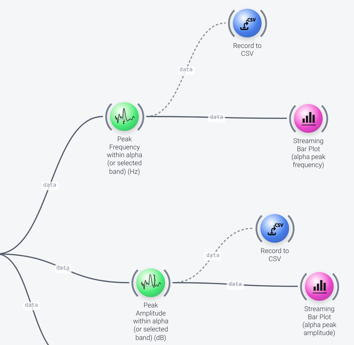
The spectrum of the selected band is passed to two nodes, which work on the frequency axis:

• The Peak Frequency node (a Peak Latency node with its axis set to frequency) outputs the frequency at which the spectrum within the band is highest, in Hz.
• The Peak Amplitude node outputs the height of that peak, in dB.

Since the input has one spectrum per channel, each of them outputs one value per channel.

Output

(See screenshot in previous section.) Each peak value goes to its own Streaming Bar Plot, one for the peak frequency (y_limits of 6 to 14 Hz) and one for the peak amplitude (y_limits of -5 to 100 dB). Each channel is shown as a separate bar. The limits are tuned for alpha, so if you select a different band, adjust them accordingly. The title of each plot is also set here.

Each peak node is also wired to a Record to CSV node, writing to ~/neuropype/outputs/peak_frequency.csv and ~/neuropype/outputs/peak_amplitude.csv (the filename property). These connections are disabled in the example, which is why the wires are dashed. To record the values to a file, right-click the wire and enable it.