Artifact removal

This example pipeline, ArtifactRemoval.pyp, shows a standard EEG cleaning workflow that removes common artifacts from an EEG stream in real time: eye movements and blinks, muscle and movement artifacts, noisy or broken channels, and high-amplitude glitches. The core of the cleaning is done by the Artifact Removal node, which uses the Artifact Subspace Reconstruction (ASR) algorithm, preceded by a Bad Channel Removal node. The raw and the cleaned data are plotted side by side so that the effect can be inspected, and the clean data is sent out over LSL for use by other applications.

This pipeline is built for live/streaming data, but can be easily adapted for offline/recorded data.

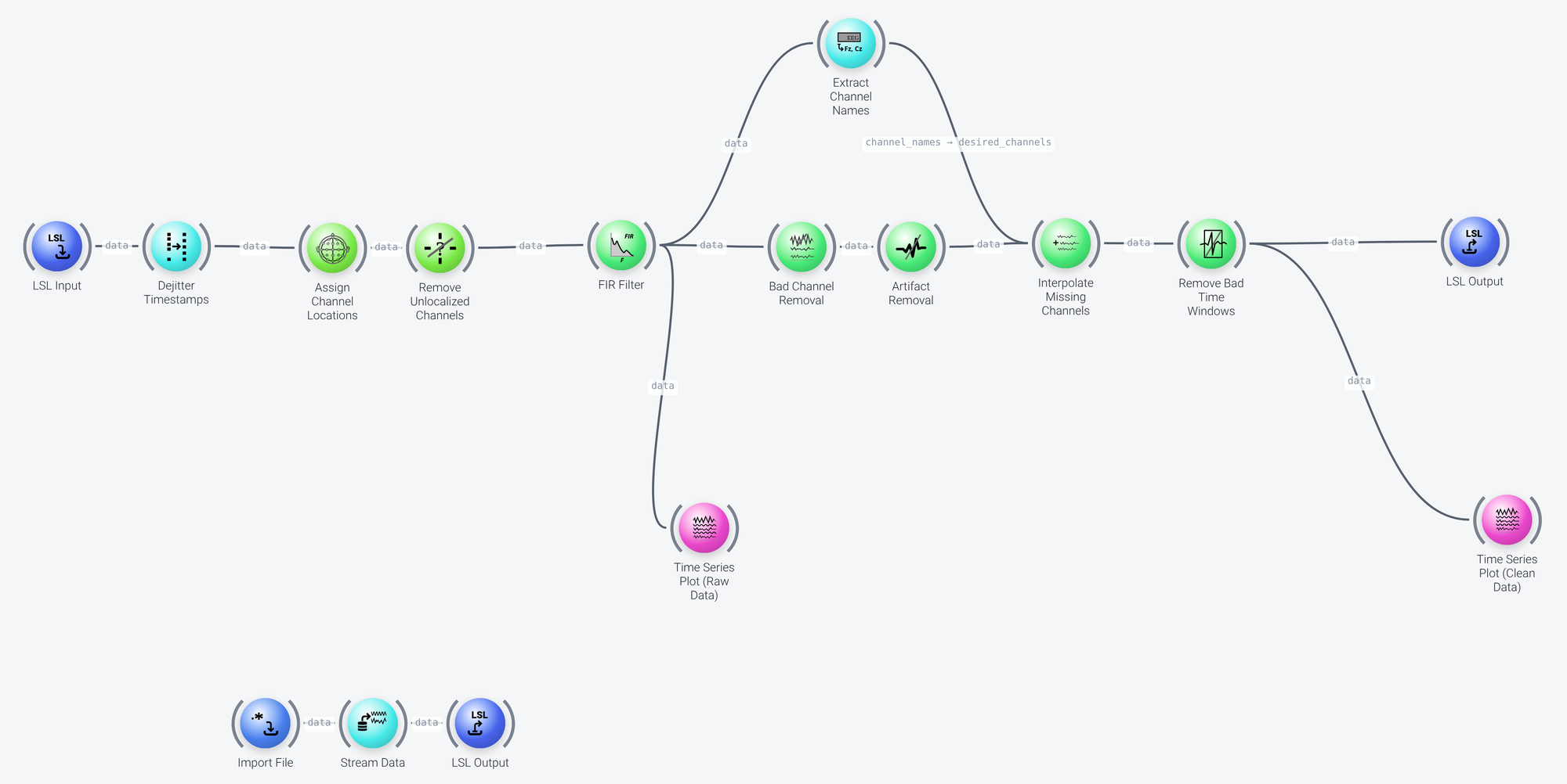
The pipeline can be divided into four parts, which we discuss in the following: data acquisition, preprocessing, artifact cleaning, and visualization and output.

Data Acquisition

Includes: LSL Input, and (for the example only) Import File, Stream Data and LSL Output

This pipeline is designed to run out of the box by restreaming recorded data. For use with live data, you would remove the playback branch and change the query property of the LSL Input node so that it finds your live EEG stream, for instance type='EEG', or the name of your device's LSL stream. For use with recorded data, change the Import File path, wire it directly into Dejitter Timestamps and drop the LSL and Stream Data nodes. See Data input in the example pipelines for details.

Preprocessing

Includes: Dejitter Timestamps, Assign Channel Locations, Remove Unlocalized Channels and FIR Filter

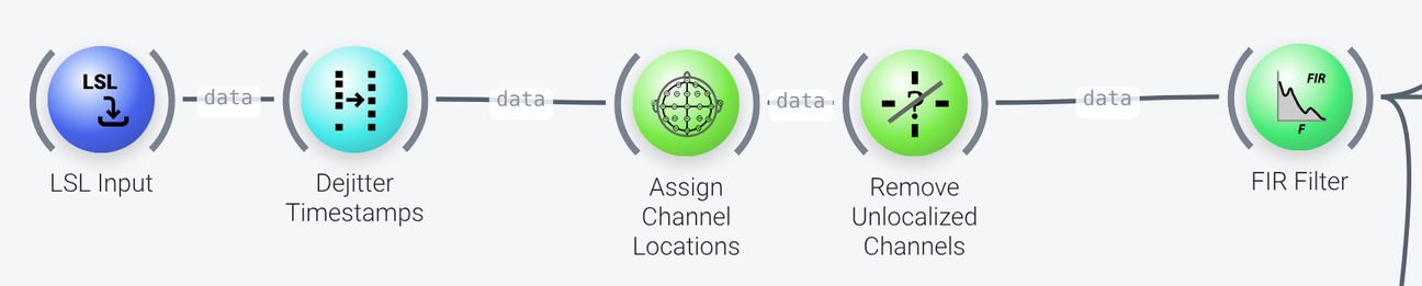
The preprocessing nodes prepare the data for the cleaning nodes:

• Dejitter Timestamps smooths out the irregularities in the time stamps of the incoming samples. You should generally always run this, unless the time stamps are generated by the EEG hardware itself. It is particularly necessary if the signal is acquired wirelessly (e.g., over Bluetooth), where samples tend to arrive in irregular bursts, which makes their time stamps jittery.
• Assign Channel Locations automatically assigns a position on the scalp to each EEG channel, looking up the default locations for channel labels in the international 10-20 system (or using a custom montage provided in its montage property). Downstream nodes need these locations, for instance the ASR uses this to determine how correlated a channel is with its neighbors.
• Remove Unlocalized Channels removes the channels that did not get a location, which are non-EEG channels such as triggers or accelerometers, since these have no position in a head montage. Removing these is essential for downstream nodes which expect EEG only, to operate properly.
• The FIR Filter is set up as a high-pass filter (frequencies of 0.5 and 1 Hz) that removes slow drifts. This is required, since the Bad Channel Removal and Artifact Removal nodes assume that the data has already been high-passed. Depending on your headset and your use case, you may want to use a lower cutoff here (e.g., 0.5 Hz or even 0.1 Hz).

Artifact Cleaning

Includes: Bad Channel Removal, Artifact Removal, Extract Channel Names, Interpolate Missing Channels and Remove Bad Time Windows

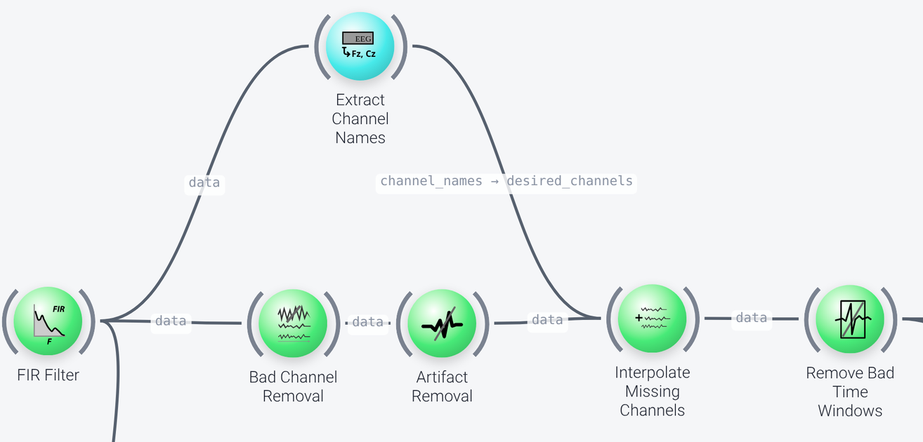
The cleaning is done in four steps, in the order in which the nodes appear in the screenshot:

• Bad Channel Removal drops channels that are outliers, so that a single broken or noisy electrode does not degrade the result. A channel is dropped if it correlates poorly with what would be expected given the other channels (the corr_threshold property, 0.8 here; higher values are more stringent, and values below 0.6 are very lax), or if it contains too much high-frequency noise (the noise_threshold property, 4 here, in standard deviations; lower values are more stringent, and values above 5 are very lax). Running this node before Artifact Removal gives better results.
• Artifact Removal removes high-amplitude artifacts using the ASR algorithm. Portions of the data whose amplitude exceeds the cutoff property (7.5 standard deviations here, relative to the calibration data) are considered artifacts and are reconstructed from the rest of the signal. Lower values are more aggressive and and would attenuate some large but genuine EEG phenomena, while values between 10 and 15 preserve most of the EEG signal. Typically higher values (less aggressive) are preferred for data that has a lot of motion artifacts. ASR works best with higher-density montages (19 channels and up), though it can be used with as few as 4 channels.
• Interpolate Missing Channels restores the channels that Bad Channel Removal dropped, by interpolating them from the remaining channels, so that the output has the same channels as the input. The list of channels it should produce comes from the Extract Channel Names node, which reads the channel names from the data before any channels were removed and passes them on to the desired_channels property of the interpolation node.
• Remove Bad Time Windows drops the time segments that are still outliers after cleaning with ASR. Its zscore_thresholds property (-4 and 6 here) sets the amplitude range that counts as normal, and the max_bad_channels property (0.2 here) sets the fraction of channels that may be outside this range before a window is dropped. Note that this only works on recorded data, not live data, so this node has no effect when the pipeline is run on a live stream.

Calibration

Bad Channel Removal and Artifact Removal need clean(-ish) baseline data to calibrate their algorithms. When processing a stream, each of them buffers the first few seconds of data (the calib_seconds property of each node, 30 seconds by default) before it starts to output clean data, so the cleaned output only appears after this initial period. When processing offline data, these nodes calibrate on the entire data set instead.

Visualization and Output

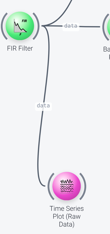
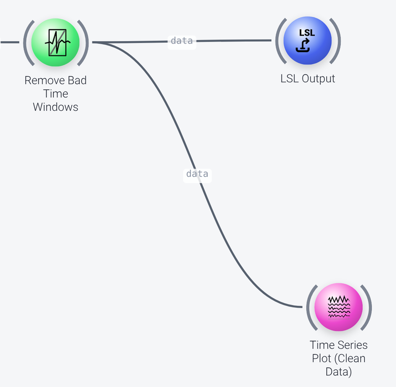
The pipeline has two Time Series Plot nodes so that the data before and after cleaning can be compared. Time Series Plot (Raw Data) is fed from the FIR Filter (the first screenshot above), and Time Series Plot (Clean Data) from the end of the cleaning chain (the second screenshot). Both show the last 5 seconds of data (the time_range property) and up to 19 channels (max_channels), and each has its own window title.

The cleaned data is also sent to an LSL Output node, which makes it available as an LSL stream named CleanedEEG (its stream_name property), so that it can be picked up by other applications. This is a different name from that of the input stream, MyOutputStream.

You may also want to save the cleaned data to disk, in which case a Record to XDF node can be wired to the end of the cleaning chain, whether the data is live or recorded. When working with recorded data, drop the LSL Output node. The Time Series Plot nodes would still work, but since they try to plot the entire recording in one figure, they will be very slow to load if the recording is large, so not recommended in that case. What you could do is to preface the plot with a Select Range node to select a portion of the recording along the time axis and then plot that.