Conditional workflow with exposed parameters

This example pipeline, ConditionalWorkflow.pyp, illustrates two concepts:

• using the If / Else node to control the flow of execution, in this case whether a node (here the Re-referencing node) is executed or not, depending on the value of a parameter;
• using ParameterPort nodes to expose parameters that can be set at runtime, for instance over the NeuroPype API, without having to load and edit the pipeline.

The rest of the pipeline is a simple spectral analysis: the data is band-pass filtered, optionally re-referenced, and its power spectrum is computed over a sliding window and plotted.

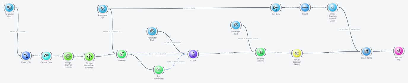
The pipeline can be divided into five parts, which we discuss in the following: data acquisition, exposed parameters, preprocessing, the conditional branch, and the spectrum computation and plot.

Data Acquisition

Includes: Import File, Stream Data, Assign Channel Locations and Remove Unlocalized Channels

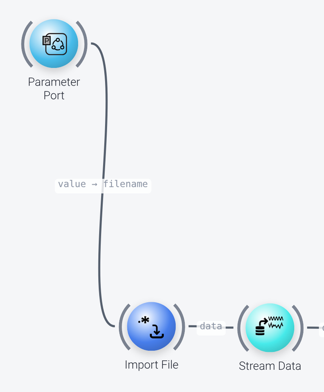
The pipeline loads a recording with the Import File node and streams it with the Stream Data node, to mimic a live data stream (the file here is VisualArrest.xdf). To use live data, you would replace these two nodes with an LSL Input node. See Data input in the example pipelines for more on this.

The Assign Channel Locations and Remove Unlocalized Channels nodes, which are shown in the next screenshot, assign scalp locations to the EEG channels and remove the channels that have no location, i.e., non-EEG channels, such as triggers.

Exposed Parameters

The pipeline has four ParameterPort nodes. Each of them defines a parameter of the pipeline that is exposed to the outside, and passes its value on (through its value port) to a property of another node. The parameters of a pipeline can be set when the pipeline is launched, for instance in Pipeline Desinger, from the NeuroPype Control Panel (where all the parameter ports of a selected pipeline are displayed), from the command line, or from another application over the NeuroPype API. See the tutorial on exposing parameters with ParameterPorts for more on this.

Here, the parameter ports expose the following parameters:

portname	Passed to	value_type	default
input_file	the filename property of Import File	string	MotorImageryTrain.set
frequencies	the frequencies property of FIR Filter (and the frequency range of the plot)	list[float]	[0.25, 0.5, 45, 50]
use_rereference	the condition port of If / Else	bool	True
window_len	the window_length property of Moving Window	float	2

It is good practice to document your parameter ports fully, and to specify both the correct data type and a helpful default value. Besides portname, value_type and default, the properties that you will want to set on a parameter port are its desc (a description, shown in the applications that display the parameter), its verbose_name (a human-friendly name, such as Input File) and its port_category (the group under which the parameter is shown, here Input Data, Processing or Spectral). Properties such as is_filename (for file paths), is_visible and editable control how the parameter behaves in client applications.

Preprocessing

Includes: Assign Channel Locations, Remove Unlocalized Channels and FIR Filter

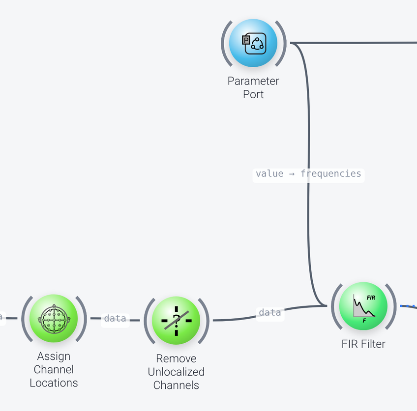
The FIR Filter is a band-pass filter, and its frequencies property is not set in the node, but comes from the frequencies parameter port above it. The four values are the edge frequencies of the filter, in Hz (here 0.25, 0.5, 45 and 50), so that the pass band is from about 0.5 to 45 Hz.

The Conditional Branch

Includes: Re-referencing and If / Else

Since a pipeline is a graph, branching works differently from what you may be used to in a programming language. There is no node that tests a condition and then has two branches leading away from it to the nodes downstream. Instead, the two alternative branches both start at the same upstream node, and come together again in the If / Else node at their end. This node evaluates the condition, goes back to and runs only the branch that it selects, and passes the output of that branch on to the node(s) downstream of it. The wires that connect the branches to the If / Else node are dotted, instead of solid, to indicate that they are dependant on another node (If/Else in this case).

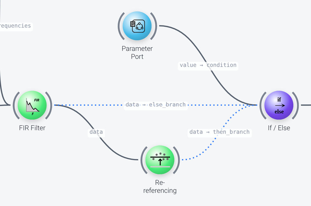
After the filter, the flow of execution either goes through the Re-referencing node or bypasses it, depending on the value of the use_rereference parameter. This is done by the If / Else node, which has a condition port (wired to the parameter port) and two branches, the then_branch and the else_branch:

• If the condition is true, the data goes from the FIR Filter through Re-referencing (which here performs common average referencing, i.e., subtracts the average of all channels, as set by its reference_range of :) and on to the If / Else node, which passes the result on through its result port.
• If the condition is false, the data goes directly from the FIR Filter into the else_branch of If / Else, which passes it on unchanged.

As mentioned above, the If / Else node is at the end of the branches, the execution works backwards from it: when the pipeline reaches the node, the execution is sent back to the branch that the condition selects, either the one wired into its then_branch or the one wired into its else_branch, and once the node receives the data resulting from that branch, it passes it on to the next node. The branch that is not taken is not evaluated, i.e., its nodes do not run. The condition is evaluated following the rules of Python, so that an empty list, an empty string and zero also count as false. If nothing is wired into the condition, the else_branch is taken.

Spectrum Computation and Plot

Includes: Moving Window, Power Spectrum (Welch), Select Range and Spectrum Plot

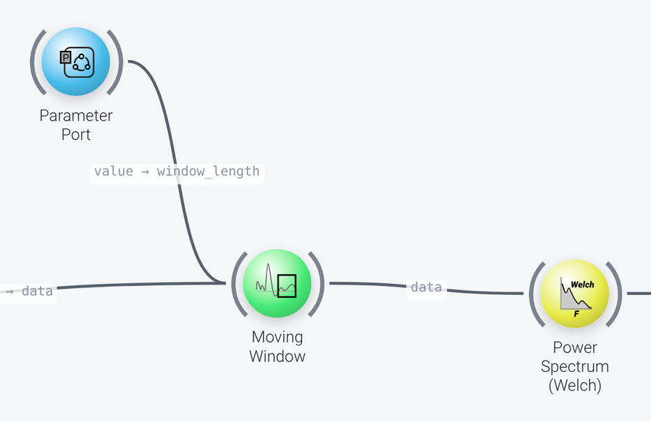
A spectrum must be computed over windows of a certain length, not over continuous data. The Moving Window node therefore segments the stream into windows, and its window_length property comes from the window_len parameter port (2 seconds by default). The Power Spectrum (Welch) node then computes the power spectral density of each window.

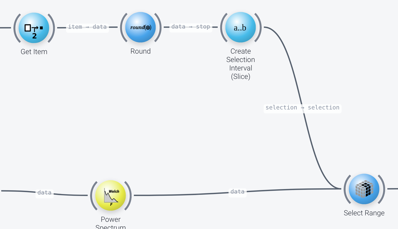
The frequency range that is shown on the Spectrum Plot is also set dynamically from a parameter, in the three nodes shown in the next screenshot. The Get Item node takes the last value of the list of frequencies from the frequencies parameter port (its key is -1), the Round node rounds it, and the Create Selection Interval (Slice) node creates a range that has this value as its stop value, which here is 0 to 50. This range is fed into the selection property of a Select Range node, which works on the frequency axis, so that the plot always shows the spectrum up to the upper edge of the filter, whichever frequencies are set.

The Spectrum Plot at the end of the pipeline shows the resulting spectrum (with a unit of PSD, and the 1/f correction enabled by one_over_f_correction).