Save data to CSV

This example pipeline, SaveToCSV.pyp, shows how to export multi-dimensional processed EEG data to a CSV file. It imports a recording, computes a spectrogram (a time-frequency representation) of two channels, selects a range of frequencies and of time from it, and saves the result to a CSV file. It also shows how multi-dimensional data is laid out in a CSV file, which is a flat table.

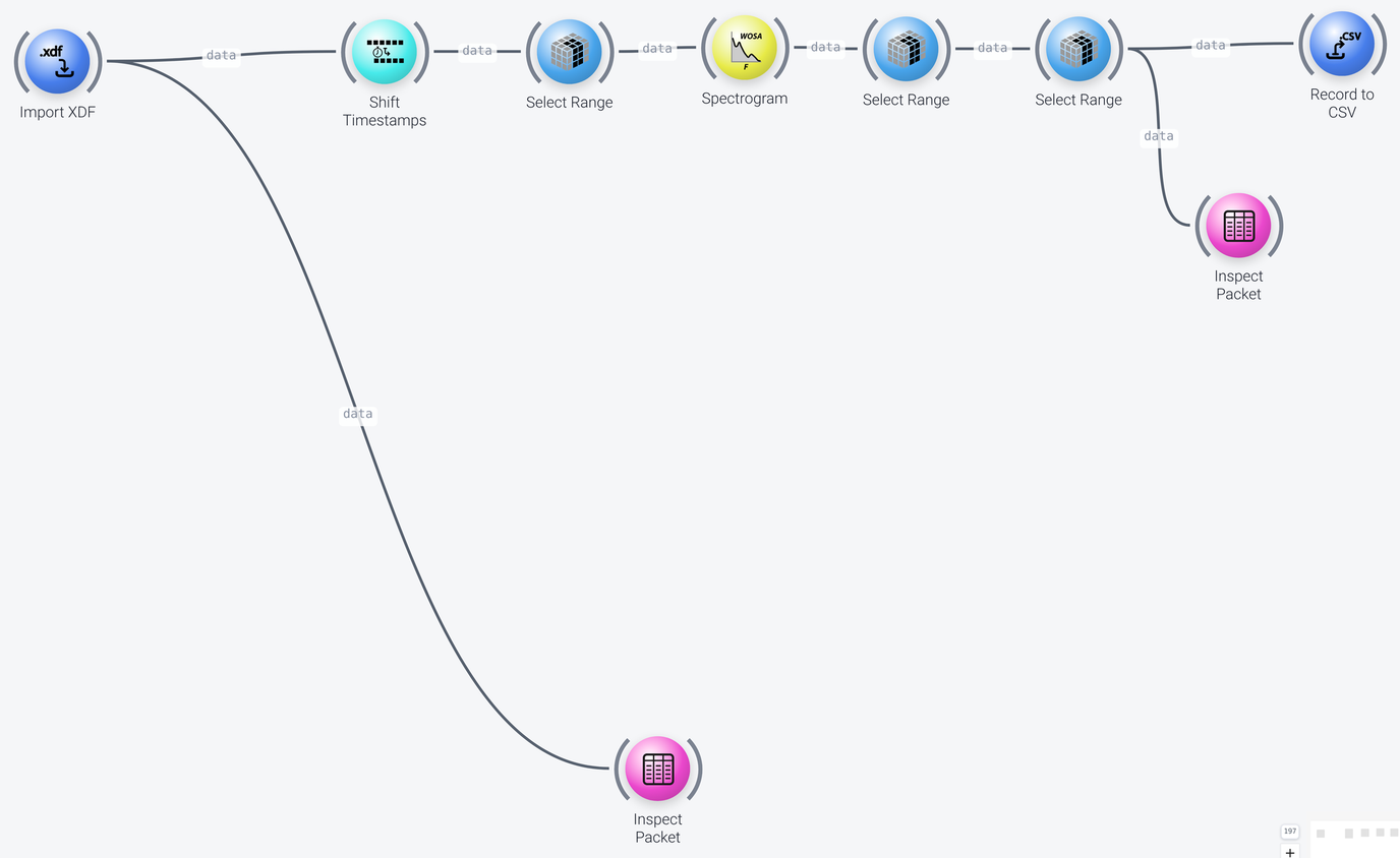
The pipeline can be divided into three parts, which we discuss in the following: importing and processing the data, selecting the data to save, and saving it.

Importing and Processing the Data

Includes: Import XDF, Shift Timestamps, Select Range, Spectrogram and Inspect Packet

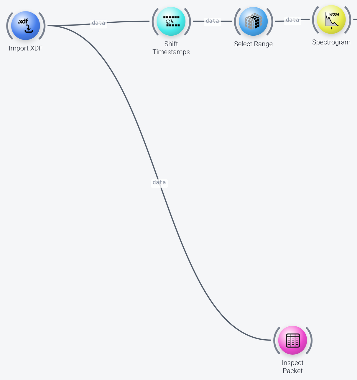
The pipeline imports a recording, the example file VisualArrest.xdf (the filename property of Import XDF). The imported data is also sent to an Inspect Packet node (the one in the bottom of the pipeline), which shows the structure and the contents of the data that comes in (see the inspect file data example for more on this node).

• Shift Timestamps shifts the time stamps of the data so that they are relative to the start of the data (the beginning_from_zero property is enabled), so that we can later select the first N seconds of the data without needing to know the time stamp at which the recording starts.
• The first Select Range node keeps two channels, Fz and Pz (the selection property, on the space axis, using names).
• Spectrogram computes a time-frequency representation of the data, using the short-time Fourier transform: the spectrum is computed for successive segments of 1 second (segment_samples of 1.0, with the unit set to seconds). The result has a new frequency axis, in addition to the time and the space axes. (This node is designed to work on offline data, unlike the Power Spectrum nodes which operate on live data.)

Selecting the Data to Save

Includes: Select Range

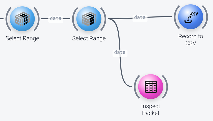
Two further Select Range nodes select a range of each of the other axes, so that the result is a small matrix with the axes space, frequency and time, which has 2 x 3 x 19 elements. The first of them keeps the frequencies from 2 to 4 Hz (selection of 2...4, on the frequency axis, with the unit set to Hz), and the second keeps the first 10 seconds (:10, on the time axis, in seconds). (Alternatively, you could select by indices instead of by names, in Hz or in seconds.)

An Inspect Packet node shows the data that is going out, with the frequency axis as its col_axis, so that you can see the structure and the contents of the data that is going to be saved.

Saving the Data

Includes: Record to CSV

The data is saved to a CSV file by the Record to CSV node. The name of the file is set by its filename property (here test-result.csv), and the folder by its output_root property.

A CSV file is a flat table, so the node lays out the data as follows: the time axis is written as rows, and the values of the time stamps are added as the last column of the file, labeled timestamp (set by the time_stamps and timestamp_label properties). The remaining axes, space and frequency axes, are automatically vectorized into a flat list of columns, one for each combination of channel and frequency. For this example, the result is a CSV file with 19 rows, and 6 + 1 columns (2 channels x 3 frequencies, plus the time stamp).

This example saves offline (recorded) data to disk. The same principle can be used to save streaming (live) data, for which the Record to CSV node is the appropriate node, since it continuously appends the data that it receives to the file. For a recording that is processed as a whole, as it is here, you can also use the Export to CSV node, which writes the entire data set at once. See the tutorial on streaming vs. offline data for more on getting data in and out.