Segment extraction

This example pipeline, SegmentExtraction.pyp, shows the typical steps that are needed to extract segments (also called trials or epochs) from a data stream, around specific event markers. This is an essential preprocessing step if your algorithm includes machine learning techniques with supervised learning, which require target values for the different trials of data for training. In this simple example, a segment of data is extracted around each incorrect and each correct marker, after a band-pass filter, and the spectrum of the segments is computed. The raw data of the segments and the spectrum are plotted, and the spectrum is also saved to a CSV file.

These segments are typically processed further, for instance perform machine learning classification, compute statistics, send them over LSL, plot or record them to disk.

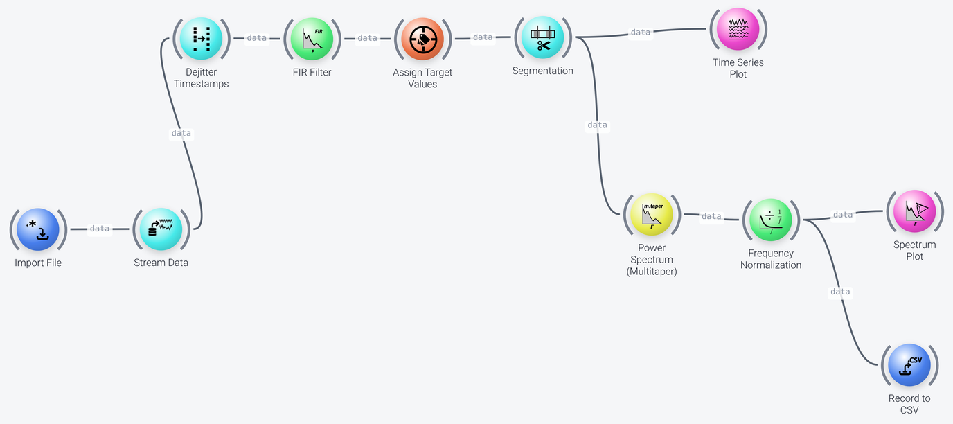
The pipeline can be divided into four parts, which we discuss in the following: data acquisition and filtering, segment extraction, spectrum computation, and output.

Data Acquisition and Filtering

Includes: Import File, Stream Data, Dejitter Timestamps and FIR Filter

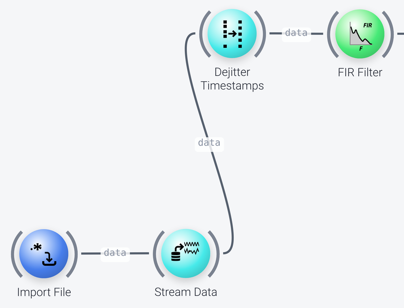
So that the example can run without a live data source, the pipeline imports a recording with the Import File node (here FlankerTest.set, set by its filename property) and plays it back with the Stream Data node, as if it were streaming. For use with live data, replace these two nodes with an LSL Input node. See Data input in the example pipelines for more on this.

Dejitter Timestamps corrects the time stamps of the incoming samples, which prevents unwanted behavior in the downstream nodes. The FIR Filter is set up as a high-pass filter (mode of highpass, with frequencies of 1 and 2 Hz), which removes slow drifts from the data before the segments are extracted.

Segment Extraction

Includes: Assign Target Values, Segmentation and Time Series Plot

• Assign Target Values (also called Assign Targets) selects the markers around which the segments are cut, and assigns a target value to each of them. It is mainly used if the pipeline includes supervised learning algorithms, and you need to know the labels of the markers in your data beforehand. Its mapping property assigns the value 0 to the marker incorrect and the value 1 to the marker correct (the mapping_format is names, and is_categorical is enabled). You can use wildcards in the mapping, for instance left* to find all the markers that start with left, by setting the mapping_format property to wildcards. If you do not need to assign classes to your event markers, you can simply specify the list of markers to segment around in the Segmentation node itself, and drop Assign Target Values.
• Segmentation extracts the segments. In the marker-locked mode (its online_epoching property), a window around each of the markers is extracted, here from 0.5 seconds before to 0.5 seconds after the marker (time_bounds of -0.5 and 0.5), so that the segments are 1 second long. In the sliding mode, a single sliding window that lies at the end of the data is extracted instead. The node resets the time axis of the segments so that it is relative to the marker, so that 0 in the time axis represents the marker.
• A Time Series Plot shows the extracted segments (it has a title of 1 second segment (0 = marker) and a time_range of 1 second, and its no_concatenate property is enabled so that every segment is shown separately). Note that the x-axis is relative to the marker.

Spectrum Computation and Output

Includes: Power Spectrum (Multitaper), Frequency Normalization, Spectrum Plot and Record to CSV

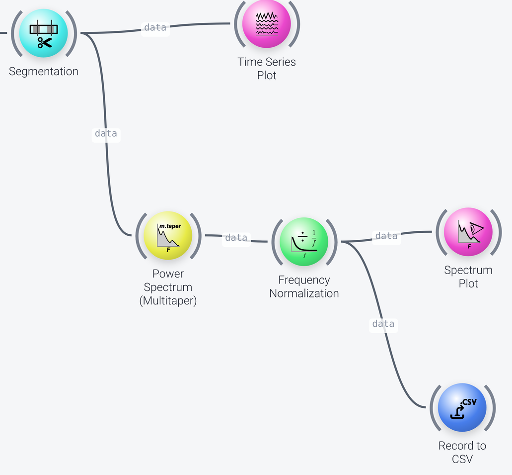
The Power Spectrum (Multitaper) node computes the power spectrum of each segment. The data now has a frequency axis. Frequency Normalization corrects the spectrum for the 1/f fall-off, and the result is shown on a Spectrum Plot. The Spectrum Plot also has an option to do the 1/f correction itself (one_over_f_correction), as an alternative to the Frequency Normalization node.

The spectra are also saved to a CSV file by a Record to CSV node, whose filename is segment-test.csv (in the folder set by its output_root property).