Streaming signal quality assessment

This example pipeline, SignalQualityAssessment.pyp, displays a number of different quality metrics for a live stream of EEG data. It receives the signal from an LSL stream, and the Channel Diagnostics node computes four quality metrics for it, and displays each of them in a plot (as a topography plot of the channels on the scalp). These are:

• the line noise of each channel (at the frequency of the mains power, 50 or 60 Hz),
• the correlation of each channel with the other channels,
• the high-frequency noise of each channel, and
• a single, weighted bad channel classification, which combines the other metrics (and the impedance, if it is provided) and classifies each channel as good, acceptable or bad.

The pipeline also includes:

• a plot of the impedance values of the channels, if the device sends an impedance stream,
• a window that shows the incoming event markers, if the data has any,
• a time series plot of the incoming data.

The plots can be switched on and off with parameter ports, and the stream names and the channels can be configured with parameter ports as well, so that the pipeline can be set up when it is launched, without editing it.

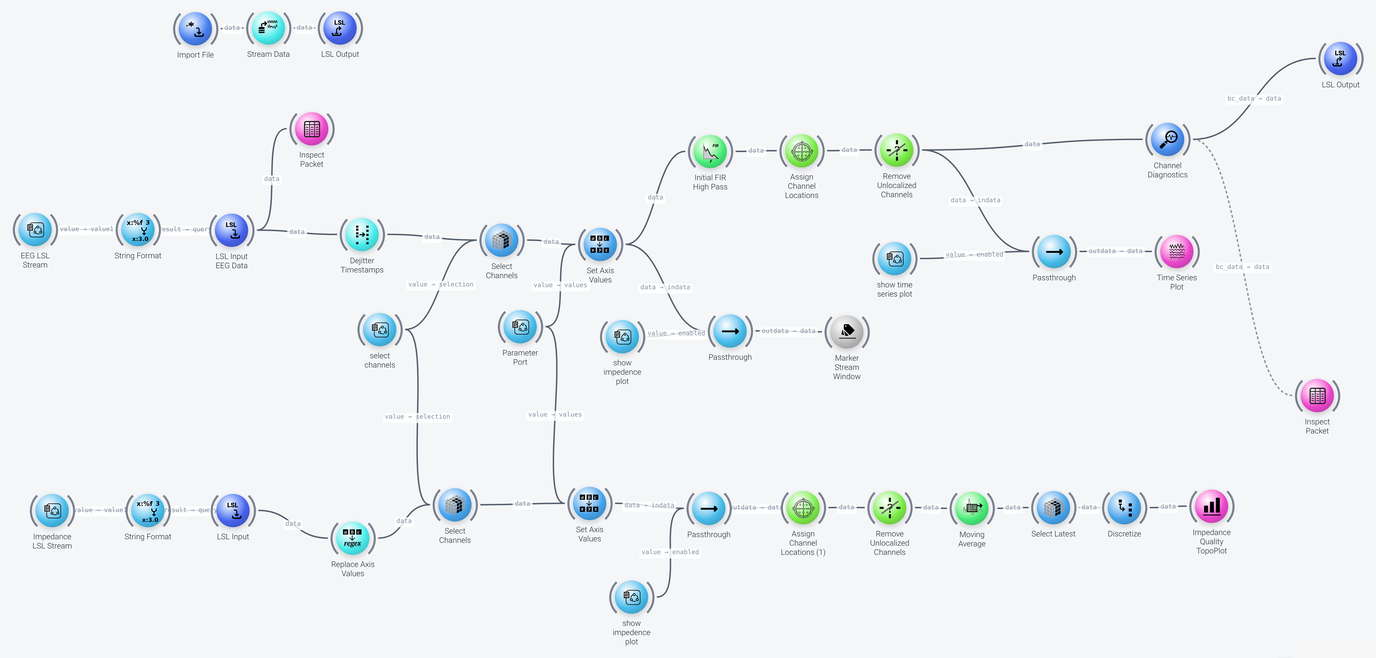
The pipeline can be divided into six parts, which we discuss in the following: data acquisition, channel selection and renaming, the signal quality metrics, the time series plot, the marker window, and the impedance plot.

Data Acquisition

Includes: Parameter Port, String Format, LSL Input and Dejitter Timestamps

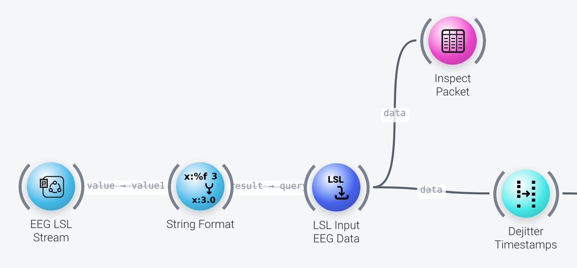
The pipeline receives its EEG data from the lab streaming layer through the LSL Input node (named LSL Input EEG Data). The name of the stream to look for is not typed into the node, but is a parameter of the pipeline: the Parameter Port named EEG LSL Stream (with the portname eeg_lsl_stream_name, and the default MyStream) holds the name of the LSL stream with the signal data. A String Format node (with a string of name='%s') inserts it into a query string, which is wired into the query property of LSL Input. The marker_query property of LSL Input is type='Markers', so that a marker stream, if there is one, is received as well. Dejitter Timestamps then corrects the time stamps of the data. An Inspect Packet node (titled Raw Data) is attached to the output of LSL Input, so that you can see the incoming channel names and data.

So that the example can be run "out of the box" without a live data source, the three nodes at the top of the pipeline (Import File, Stream Data and LSL Output, in the screenshot of the whole pipeline) play back a recording as an LSL stream called MyStream. Remove them to use the pipeline with your own live LSL stream. See Data input in the example pipelines for more on this.

Channel Selection and Renaming

Includes: Select Range and Set Axis Values, and two Parameter Port nodes

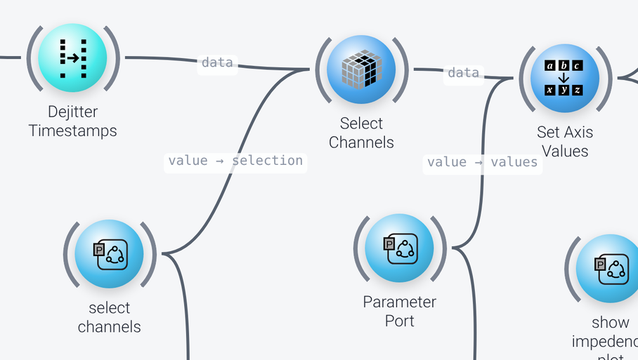
These two nodes can be used to optionally select channels, and to replace the incoming channel names if needed. A Select Range node (named Select Channels) selects the channels, with its selection property taken from the parameter port select channels (select_channels, which is (all) by default). Use this to filter out the channels that do not carry signal. A Set Axis Values node, working on the space axis, overrides the names of the channels, with the values taken from the parameter port rename_channels (an empty list by default). Use this if your device uses non-standard channel names, to give them names that match a standard montage, which is required for the locations to be assigned.

Signal Quality Metrics

Includes: FIR Filter, Assign Channel Locations, Remove Unlocalized Channels and Channel Diagnostics

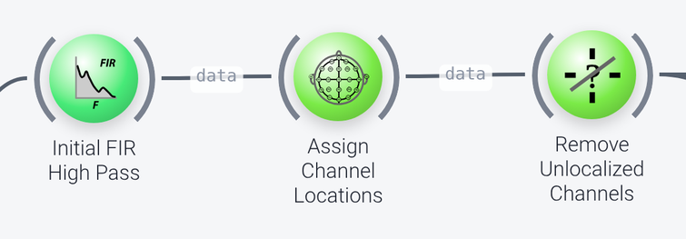
The data is first high-pass filtered by the FIR Filter (named Initial FIR High Pass, frequencies of 0.5 and 1 Hz), and Assign Channel Locations and Remove Unlocalized Channels assign a location on the scalp to each channel, based on standard montages (a custom montage can also be specified), and remove the channels that have no location (were not found in the montage), i.e., non-EEG channels, i.e., aux channels, etc. This is essential as the quality metrics are for EEG channels only.

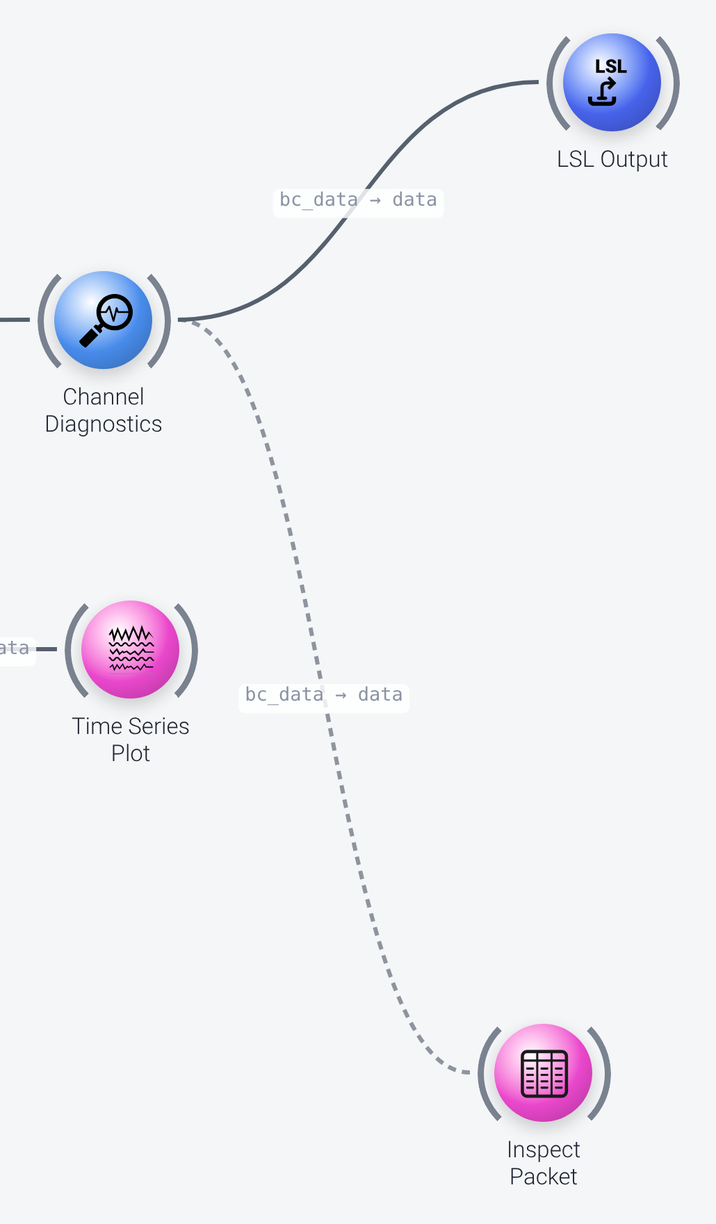
The Channel Diagnostics node computes four quality metrics, and launches a plot for each of them. It calls several other nodes to compute the line noise, the channel correlation and the high-frequency noise, and displays them as topography plots, together with a single weighted bad channel classification metric, which is also displayed as a topography plot. In the bad channel classification, each channel is marked as good (1, green), acceptable (2, yellow) or bad (3, red), depending on whether any of the following metrics is beyond its thresholds: the channel correlation (the min_corr property, 0.7 and 0.8 here), the high-frequency noise (hf_thresh, 3 and 4), and the impedance, if an impedance stream is provided to the node (impedance_thresh, 1000 and 2500). If only the high-frequency noise is bad, the channel is set to 4 and shown in purple, to distinguish channels that are bad because of high-frequency noise, which may not be easy to remedy, from channels that are bad because of poor contact, which may be. The line_noise_frequency property is the frequency of the line noise (here 60 Hz; it is 50 Hz in Europe), and the exclude_line_noise property excludes this frequency from the computation of the high-frequency noise. If you do not have a separate line noise plot and rely on the bad channel classification alone, it may be preferable to set it to False.

The node also outputs the quality metrics through its ports (bc_data, cm_data, hf_data and ln_data), so that they can be connected to LSL Output nodes and picked up by another application for visualization. Here, an LSL Output node is connected to the port that outputs the bad channel data (bc_data), as a stream called BadChannelMetric (with a stream_type of Control).

Each metric is a time by space (channels) matrix with only one time point per packet. You can enable the Inspect Packet node (named Bad Channel Metric), which is connected by a dashed wire, to see it.

Time Series Plot

Includes: Parameter Port, Passthrough and Time Series Plot

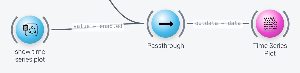
A Time Series Plot shows the incoming data of the last 10 seconds (time_range), for up to 19 channels (max_channels). It is preceded by a Passthrough node, whose enabled property comes from the parameter port show time series plot (time_series_plot, True by default). The Passthrough node passes the data through if it is enabled, and passes nothing otherwise, which turns off the nodes downstream of it. If you set the parameter to False, here or at runtime over the NeuroPype API or from the NeuroPype Control Panel, the plot is not shown.

Marker Window

Includes: Parameter Port, Passthrough and Marker Stream Window

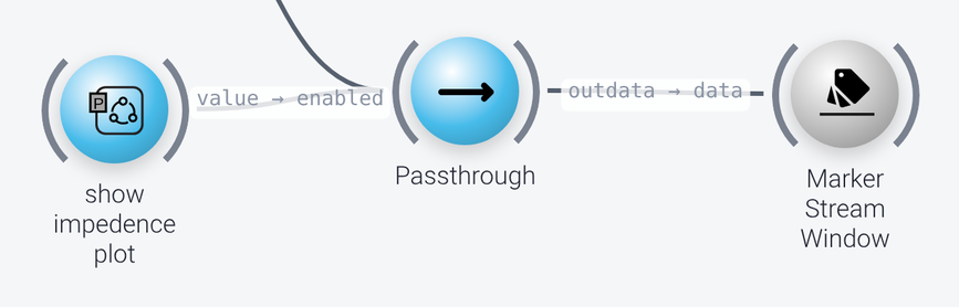
The Marker Stream Window node shows a window with the event markers and their times, as they come in, if the data has any. It is switched on and off in the same way, with a Passthrough node that is enabled by a parameter port (with the portname marker_window, which is titled show impedence plot in the pipeline).

Impedance Plot

Includes: Parameter Port, String Format, LSL Input, Replace Axis Values, Select Range, Set Axis Values, Passthrough, Assign Channel Locations, Remove Unlocalized Channels, Moving Average, Select Range, Discretize and Topography Plot

If your device outputs an LSL stream with impedance values (such as the CGX devices), you can capture it in the bottom branch of the pipeline, and plot it for quality assurance. You can also compute the impedance from the EEG data if your device supports it (see the Compute Impedance node).

As for the EEG stream, the name is a parameter of the pipeline, but you specify the type of the impedance stream, not its name (and you leave the name blank): the parameter port Impedance LSL Stream (impedance_lsl_stream_type) is formatted into the query type='%s' by a String Format node, which goes into the query property of the second LSL Input node.

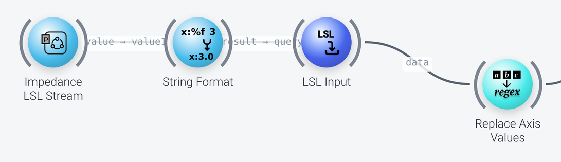
Some devices name the channels in their impedance stream differently from those in their EEG stream. For instance, Cognionics devices add a -Z suffix to the channel names. The Replace Axis Values node renames the channels using a regular expression (the pattern (.*)-Z is replaced by \1) to the standard channel names, to avoid an error in Assign Channel Locations. You probably do not need this for your data.

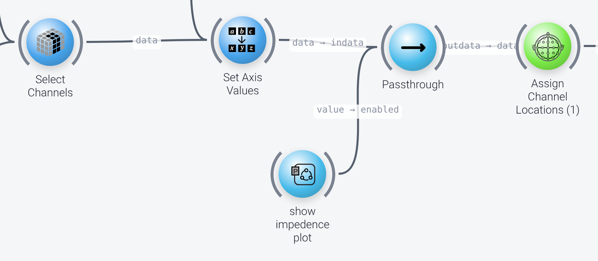
The impedance branch then selects and renames the channels in the same way as the EEG branch (the second Select Range and Set Axis Values nodes use the same parameters, select_channels and rename_channels), and then it goes through a Passthrough node, whose enabled property comes from the parameter port show impedence plot (impedence_plot, False by default). So, as for the other plots, setting this parameter to False turns the impedance plot off, and no impedance is computed or plotted. Assign Channel Locations assigns locations to the channels.

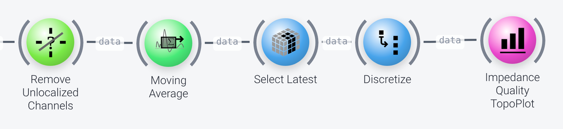
After the removal of the unlocalized channels, a Moving Average node averages the impedance over 3 seconds (order and order_unit), Select Latest keeps only the most recent value (selection of -1, on the time axis), and Discretize converts the values into three levels, 1, 2 and 3 (newvals), by two thresholds, 1000 and 2500 (threshold_cutoffs). The result is shown on an Impedance Quality TopoPlot, a topography plot of the channels on the scalp, in which the three levels are shown in the colors green, light green and red.