Time and frequency domain plotting

This simple example pipeline, TimeFrequencyDomainPlotting.pyp, computes the power spectrum of a live EEG stream and plots it, together with a plot of the EEG signal in the time domain. It is a good starting point for building your own pipelines.

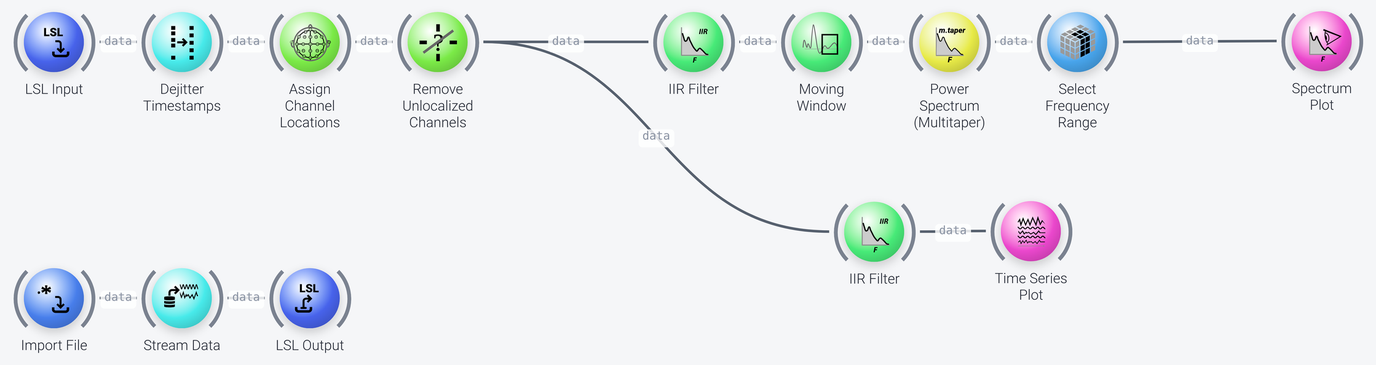
The pipeline can be divided into three parts, which we discuss in the following: data acquisition and cleanup, the spectrum plot, and the time series plot.

Data Acquisition and Cleanup

Includes: LSL Input, Dejitter Timestamps, Assign Channel Locations and Remove Unlocalized Channels

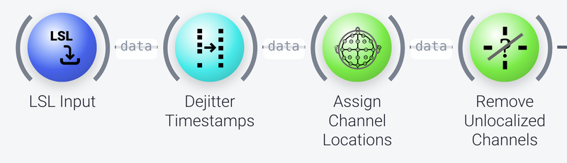
The pipeline receives its EEG data from the lab streaming layer through the LSL Input node, whose query property is set to name='MyOutputStream'. So that the example can be run "out of the box" without a live data source, the three nodes at the bottom of the pipeline (Import File, Stream Data and LSL Output, which are shown in the screenshot of the whole pipeline) play back a recording, VisualArrest.xdf, as an LSL stream with that name. For use with live data, remove them and change the query property of LSL Input so that it finds the stream of your device. See Data input in the example pipelines for more on this.

• Dejitter Timestamps corrects the time stamps of the data stream, which prevents unwanted behavior in the downstream nodes.
• Assign Channel Locations assigns a position on the scalp to each channel, based on a standard montage, and Remove Unlocalized Channels removes the channels that did not get a location. Together, they are a good way to remove the non-EEG channels (such as a reference or trigger channel) from the data.

Spectrum Plot

Includes: IIR Filter, Moving Window, Power Spectrum (Multitaper), Select Range and Spectrum Plot

• The IIR Filter is a high-pass filter (mode of highpass, a Butterworth filter, design of butter, with frequencies of 0.5 and 1 Hz) that removes the DC component of the data, but keeps the higher frequencies, so that they can be plotted in the spectrum.
• A spectrum is computed over windows of data, not over continuous data. The Moving Window node therefore outputs the most recent window of 3 seconds (window_length) on every update.
• The Power Spectrum (Multitaper) node computes the spectrum of the window with the multitaper method, which gives a high-quality spectral estimate (its half_bandwidth property sets the smoothing). This could be replaced with a Power Spectrum (Welch) node if you prefer that algorithm. Note that the Spectrogram node won't work here as that operates on offline (recorded) data.
• The Select Range node (named Select Frequency Range) retains the frequencies from 0 to 150 Hz (0...150, on the frequency axis, in Hz) and drops the rest.
• The Spectrum Plot shows the spectral content of the signal for the 19 channels (max_channels). It has an option to compensate for the 1/f fall-off that is inherent in natural signals (one_over_f_correction), which is enabled in this example.

Time Series Plot

Includes: IIR Filter and Time Series Plot

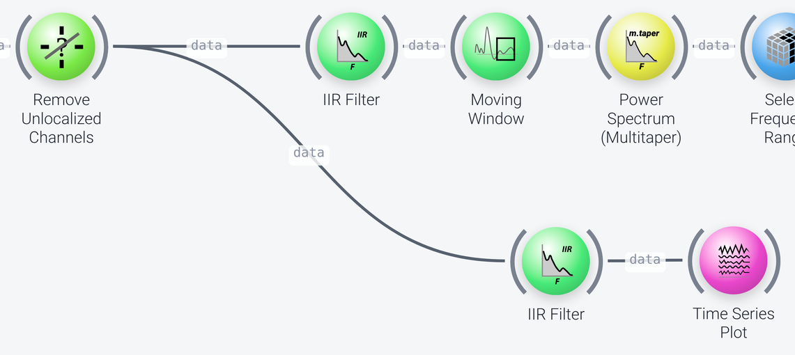
The data is also sent to a second IIR Filter and a Time Series Plot, to plot the data in the time domain. Here, the filter is a band-pass filter, with frequencies of 1, 4, 45 and 50 Hz, i.e., stop bands from 1 to 4 Hz and from 45 to 50 Hz in its frequencies property, which removes the content outside the typical frequency range of EEG. It is used to only plot the time series for frequencies up to 50 Hz, which is the range of interest here, whereas for the spectrum plot only a 1 Hz high-pass filter is used, so that the higher frequencies can be plotted. The Time Series Plot shows the last 5 seconds of the signal (time_range).