Calibrate on streaming data

This example pipeline, CalibrateonStreamingData.pyp, shows how to calibrate the adaptive and machine learning nodes of a pipeline on the fly, on the first part of a live data stream. Most machine learning nodes need to be trained on calibration data before they can make predictions. There are two general ways to provide such data: using a prerecorded file and the Inject Calibration Data node, as shown in Calibrate on prerecorded data, or collecting the calibration data at the beginning of a real-time session and using the Accumulate Calibration Data node, as in this pipeline.

The pipeline is the same classification pipeline as in the prerecorded example (it classifies EEG segments from a flanker task as correct or incorrect with logistic regression, and measures and plots its performance), with a different way of getting the calibration data. We therefore refer to that page for a more detailed discussion of the processing nodes, and focus here on what is different.

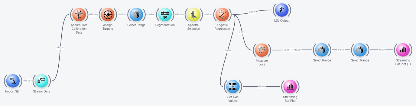
The pipeline can be divided into four parts, which we discuss in the following: data acquisition and calibration, preprocessing and classification, performance measurement, and output.

Data Acquisition and Calibration

Includes: Import SET, Stream Data and Accumulate Calibration Data

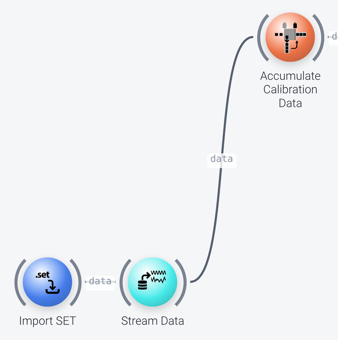
The data source of this pipeline is a single recording, FlankerTrainTest.set (the filename property of Import SET), that is played back by Stream Data (at 15 times the real-time speed, speedup) as if it were streaming data from a device. In actual use, you would replace these two nodes with an LSL Input node (and typically a Dejitter Timestamps node) that receives the stream from your device. See Data input in the example pipelines for more on this.

The Accumulate Calibration Data node buffers the first part of the stream as calibration data, and emits it in one chunk, so that the nodes after it can calibrate on it. After that, it lets the regular streaming data through, so that the pipeline can process it. For this to work, the node needs to know where the calibration data begins and where it ends. You are responsible for inserting special markers into the data, one at the beginning and one at the end of the calibration period. The strings to look for are set by the begin_marker and end_marker properties, which are the default markers calib-begin and calib-end here (with marker_mode set to markers, they are matched to the event markers in the data; the alternative, relative-times, interprets them as time offsets in seconds from the beginning of the data). Other settings used here are:

• calibration_first is enabled, so that no streaming data is emitted before the first calibration chunk has ended. This is needed for methods that can only predict once they have been calibrated.
• emit_calib_data and emit_predict_data are both enabled, so that both the calibration data and the data outside the calibration markers are passed on.

Preprocessing and Classification

Includes: Assign Targets, Select Range, Segmentation, Spectral Selection and Logistic Regression

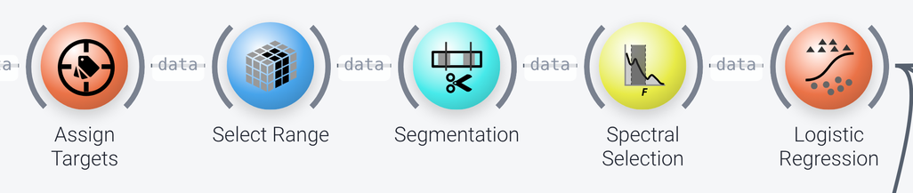
These nodes are the same as in the prerecorded example: Assign Targets assigns the target value 1 to the marker incorrect and 0 to the marker correct, Select Range keeps the first 20 channels, Segmentation cuts segments from 0.2 seconds before to 0.8 seconds after each marker, Spectral Selection band-pass filters the segments to 0.1 to 15 Hz, and Logistic Regression classifies them. The logistic regression node is trained on the calibration data that the Accumulate Calibration Data node emitted first (see Calibrate on prerecorded data for a more detailed discussion of the properties of these nodes).

Performance Measurement

Includes: Measure Loss and two Select Range nodes

The Measure Loss node computes the misclassification rate (MCR), and the two Select Range nodes select the loss value and its standard error (the value and se_stat entries of the statistic axis) and the MCR metric (from the feature axis). The result is plotted on a Streaming Bar Plot with its axis property set to statistic. Note that the loss is taken from the loss output port of Measure Loss, not from its data port.

Output

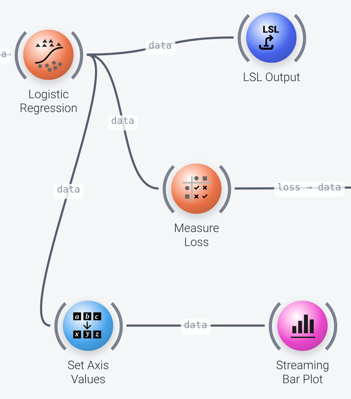
The predictions of the Logistic Regression node are sent out over LSL by an LSL Output node (with a stream_type of Control), so that they can be picked up by another pipeline or application. They are also plotted on a Streaming Bar Plot, after a Set Axis Values node has given the two classes their names (correct and incorrect) on the feature axis.