Calibrate on prerecorded data

This example pipeline, CalibrateonPrerecordedData.pyp, shows how to calibrate the adaptive and machine learning nodes of a pipeline on prerecorded data, before the pipeline starts processing live data. Most machine learning nodes (and many adaptive signal processing nodes) need calibration data to train their parameters before they can make predictions. There are two general ways to provide it: using a recording, with the Inject Calibration Data node as in this pipeline, or training on the fly at the beginning of a real-time session with the Accumulate Calibration Data node, as shown in the Calibrate on streaming data example.

As an example task, the pipeline classifies EEG segments into two classes (the example data come from a flanker task, with the markers correct and incorrect) using logistic regression. The classifier is trained on one recording and then applied to a stream, and its performance is measured and plotted.

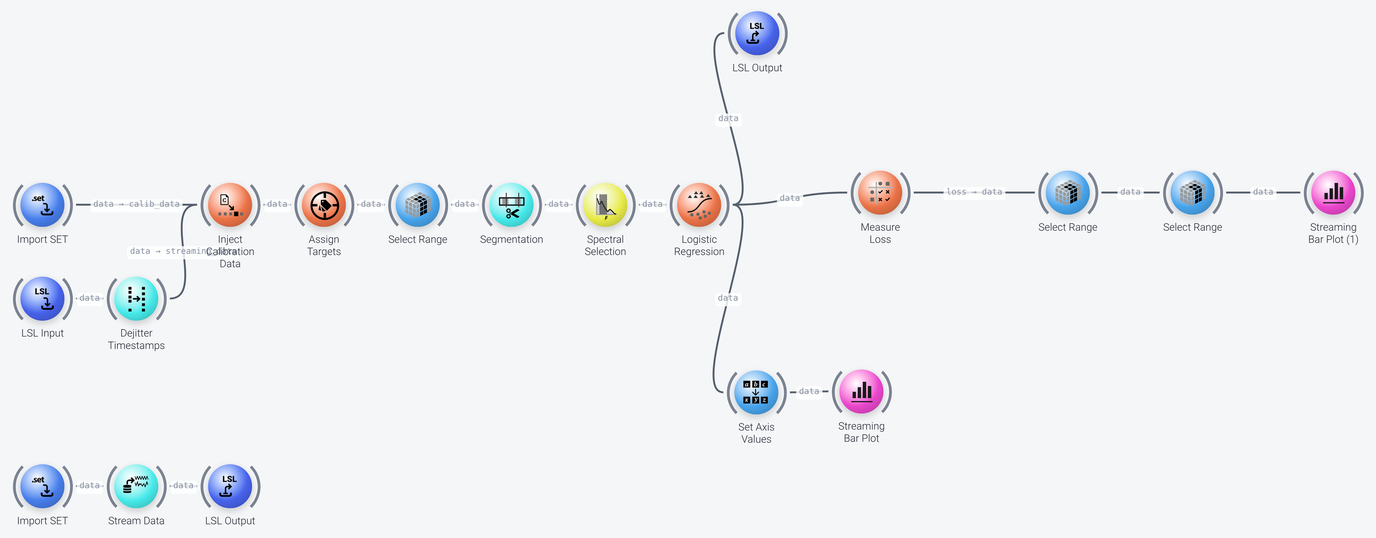
The pipeline can be divided into five parts, which we discuss in the following: data acquisition and calibration, preprocessing, classification, performance measurement, and output.

Data Acquisition and Calibration

Includes: Import SET, LSL Input, Dejitter Timestamps and Inject Calibration Data

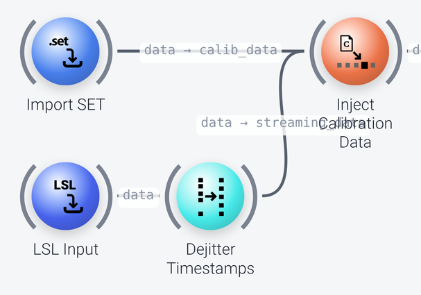
The Inject Calibration Data node sits between the data sources and the first adaptive processing step of the pipeline. It has two inputs:

• The calibration data (calib_data port), which comes from an Import SET node that loads the training recording FlankerTrain.set (its filename property). The node lets this recording through first, so that it flows down the pipeline and every node gets a chance to calibrate itself on it.
• The regular streaming data (streaming_data port), which comes from an LSL Input node followed by Dejitter Timestamps. After the calibration data has passed through, the node lets this stream through, and the pipeline processes it normally, now that it is calibrated.

The delay_streaming_packets property of the node is enabled here. The node outputs the calibration data on its first tick, so with this property enabled, it buffers the first streaming packet and emits it on the next tick (and all later packets are delayed by one tick as well), so that no streaming data is lost. If it is disabled, the first streaming packet is dropped instead. This is also the setting to use if you want to train and test the pipeline on files, without a streaming node.

For this example, the streaming data is played back from a second recording, FlankerTest.set, by the nodes in the bottom row of the pipeline: Import SET loads it, Stream Data plays it back (at 5 times the real-time speed, speedup), and LSL Output sends it out as a stream called MyOutStream, which the LSL Input node finds with its query property (name='MyOutStream'). This pipeline needs event markers, so the LSL Output node has its send_markers property enabled, which sends the markers as a second stream called MyOutStream-markers, and the marker_query property of LSL Input is set to find that stream. See Data input in the example pipelines for more on this playback setup and for how to use your own live data. With live data, the calibration recording should come from the same device (with the same channels) as the live stream.

Preprocessing

Includes: Assign Targets, Select Range, Segmentation and Spectral Selection

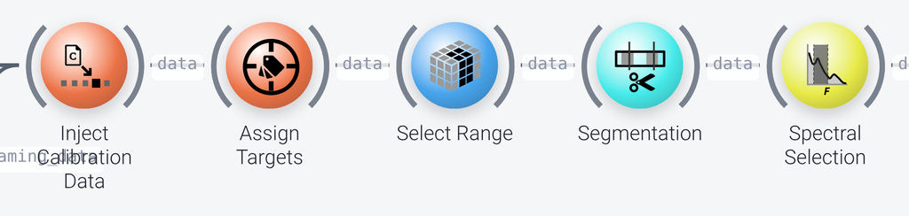
• Assign Targets selects which markers contain the event-related activity of interest and assigns a numeric target value to each. Its mapping property assigns the value 1 to the marker incorrect and 0 to the marker correct, taken from the Marker column (iv_column). The classifier needs these targets for supervised learning. You would set mapping to the marker labels in your data that correspond to the two classes you want to classify.
• Select Range keeps only some channels, here the first 20 (selection of :20 on the space axis, using indices). Use it to exclude channels that do not carry EEG, or select only a subset of EEG channels. Another method of discarding non-EEG channels is to use the Assign Channel Locations and Remove Unlocalized Channels nodes (see the Preprocessing and band power example pipeline).
• Segmentation cuts the data into segments around the markers: from 0.2 seconds before to 0.8 seconds after each marker (time_bounds). Its online_epoching property is set to marker-locked, so segments are extracted around markers in the same way for the calibration recording and for the streaming data. The alternative, sliding, would extract a single segment at the end of the streaming data on every tick.
• Spectral Selection band-pass filters the segmented data to 0.1 to 15 Hz (frequencies), which isolates the slow cortical potentials of event-related activity from higher-frequency content.

Classification

Includes: Logistic Regression

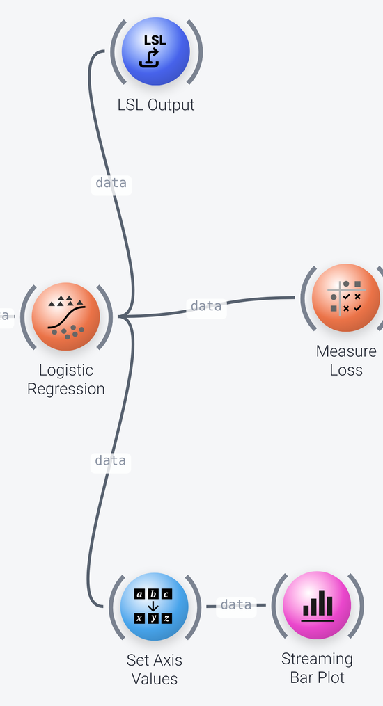
The Logistic Regression node performs the classification. On the calibration data, it is trained with supervised learning, using the target values assigned earlier (cond_field property of TargetValue node). The chosen regularization here is l2 (regularizer), and its strength is chosen from the candidate values in alphas by 5-fold cross-validation (num_folds), using accuracy as the criterion (search_metric). The probabilistic property is enabled, so the output consists of class probabilities. Once calibrated, the node applies the trained model to each segment of the streaming data.

Performance Measurement

Includes: Measure Loss and two Select Range nodes

The Measure Loss node compares the predictions with the true labels and computes performance measures over the incoming segments. It is set to compute two loss metrics, the misclassification rate (MCR) and the mean squared error (MSE), which is only to show how multiple metrics are computed, since only one of them is plotted. Besides the value of each metric, the node outputs statistics such as the standard error (see the node's documentation), which are on a statistic axis. To plot the result, the two Select Range nodes select the information of interest: the first keeps the value and se_stat entries of the statistic axis (the loss value and its standard error), and the second keeps the MCR metric from the feature axis. Note that the Select Range port is wired into the loss output port of Measure Loss, not from its data port, as the loss port contains the loss measures. The result is shown on a Streaming Bar Plot; its axis property should be set to the axis that is shown along the x-axis of the plot, which here is the statistic axis, since we plot multiple statistics for a single metric. If you were plotting multiple metrics (features) for a single statistic, it would be set to feature.

Output

The predictions of the Logistic Regression node are used in two ways here (see the screenshot in the Classification section). They are sent out over LSL by an LSL Output node (with a stream_type of Control), so that the classification result can be picked up by another pipeline or application. They are also plotted on a second Streaming Bar Plot, after a Set Axis Values node has given the two classes their names (correct and incorrect) on the feature axis. This bar plot shows the probability of each class, between 0 and 1 (its y_limits). You could also save them to disk (use the Record to CSV file), use them for downstream processing in the same pipeline, etc.