Cardiac measures from ECG

This example pipeline, CardiacMeasures.pyp, takes one or several ECG channels and computes the heart rate (HR), the heart rate variability (HRV) and the respiration rate (RR) from them, in real time. The ECG channels are averaged, filtered, and the R peaks of the heartbeats are detected, from which the three measures are computed in parallel. Each of them is shown on a bar plot, and the ECG signal with the detected peaks is also plotted.

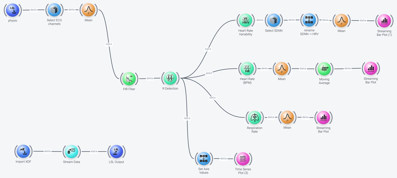
The pipeline can be divided into five parts, which we discuss in the following: data acquisition, preprocessing and R peak detection, heart rate, heart rate variability, and respiration rate.

Data Acquisition

Includes: LSL Input, and (for the example only) Import XDF, Stream Data and LSL Output

The pipeline receives its data from the lab streaming layer through the LSL Input node (the first node of the screenshot in the next section), named physio here. Its query property is set to name='physio'. The proc_dejitter and proc_monotonize properties of this node are enabled, so it also cleans up the time stamps of the incoming samples.

So that the example can be run "out of the box" without a live data source, the three nodes in the bottom row play back a recording, cgx_aim_short.xdf (the filename property of Import XDF) and restream as an LSL stream called physio. For use with live data, remove these three nodes and change the query property of LSL Input so that it finds the stream of your device. See Data input in the example pipelines for more on this setup.

Preprocessing and R Peak Detection

Includes: Select Range, Mean, FIR Filter and R Detection

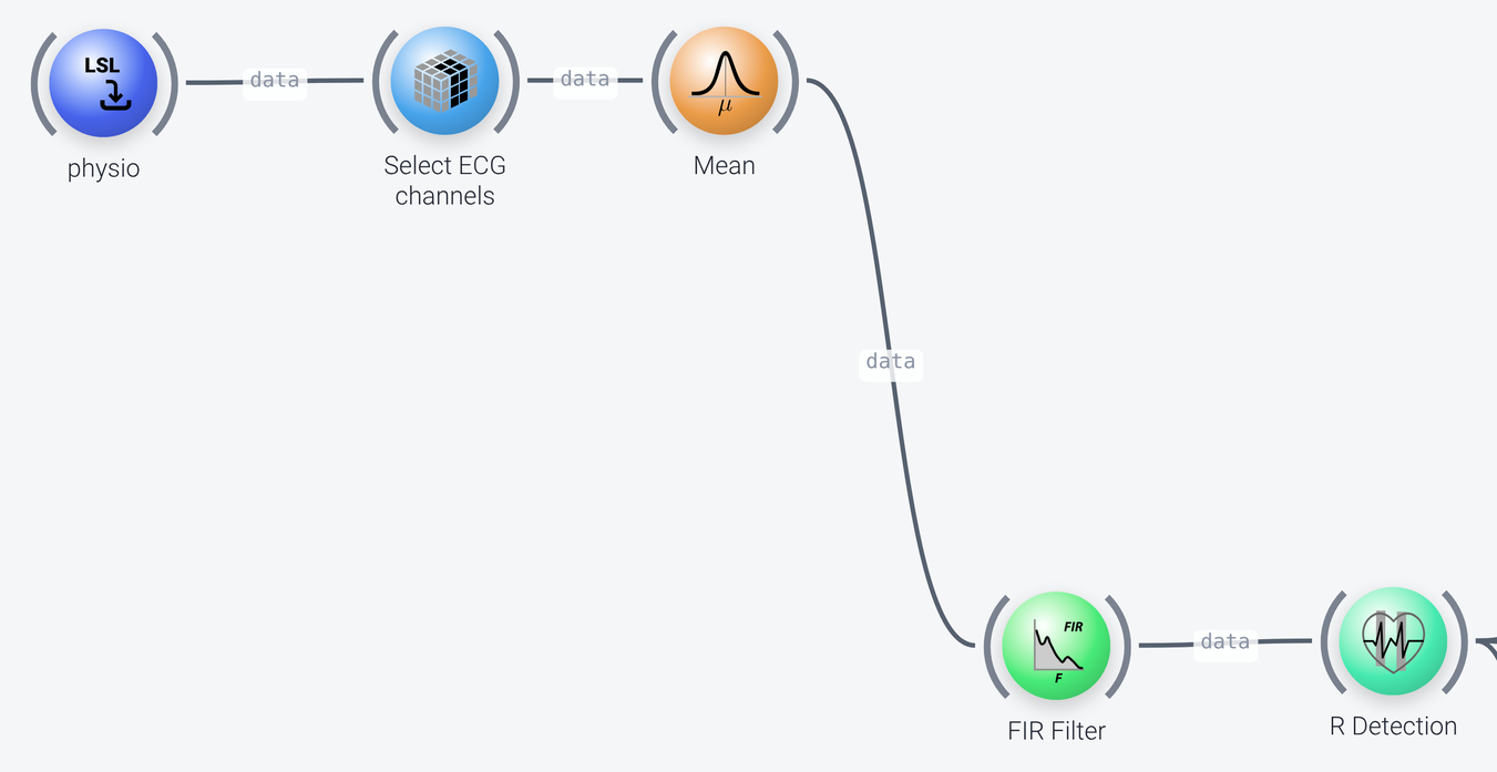
• The first Select Range node (named Select ECG channels) selects the ECG channels in the stream (the selection property, here a single channel named ExGa 1, using names). If you have multiple ECG channels, you can specify them here.
• The Mean node averages the selected channels (along the space axis) into a single channel, which is what the R Detection node expects. Note that this node names the resulting channel average.
• The FIR Filter is a band-pass filter (mode of bandpass) with the frequencies 0.5, 1, 45 and 50 Hz, which retains the signal range from about 1 to 45 Hz. A band-pass filter is used instead of just a high-pass filter, so that the signal is also cut off before any line noise.
• R Detection detects the R peaks in the QRS complexes of the ECG signal, using a modified version of the Pan-Tompkins algorithm. Its max_heartrate property (240 beats per minute here) is the highest heart rate that can be detected. The node can also detect the peaks in a PPG signal. It outputs the times of the detected peaks (together with the amplitude of the signal at these times), in a new stream whose name has -peaks appended to the incoming stream name. This output is the input of the nodes that compute the heart rate, the heart rate variability and the respiration rate. (To see the names of the streams coming out of a node, wire an InspectData node into the output port of the node in question.)

Heart Rate

Includes: Heart Rate (BPM), Mean, Moving Average and Streaming Bar Plot

The Heart Rate (BPM) node calculates the heart rate in beats per minute from the detected R peaks within a sliding window. The window is 10 seconds long (window_length and window_length_unit) and is moved by 3 seconds on every update (window_shift). The output is a stream with an irregular sampling rate, so a Mean node averages the values along the time axis into a single value per update. The Moving Average node, which averages over the last 10 seconds (order and order_unit), smooths the heart rate values to make them less noisy, and can be dropped if you do not want this. The heart rate is shown on a Streaming Bar Plot (y_limits of 40 to 140 beats per minute).

Heart Rate Variability

Includes: Heart Rate Variability, Select Range, Set Axis Values, Mean and Streaming Bar Plot

The Heart Rate Variability node calculates several measures of heart rate variability from the R peaks within a sliding window, which is 50 heartbeats long here (window_length and window_length_unit set to beats). See the documentation of the node for the full list of the measures that it calculates. This pipeline uses only the SDNN, the standard deviation of the intervals between the peaks (in milliseconds), which is selected by the Select Range node (named Select SDNN). The Set Axis Values node (named rename SDNN -> HRV) renames this feature to HRV, and a Mean node averages the values along the time axis into one value per update. The result is shown on a Streaming Bar Plot (y_limits of 50 to 300).

Respiration Rate

Includes: Respiration Rate, Mean and Streaming Bar Plot

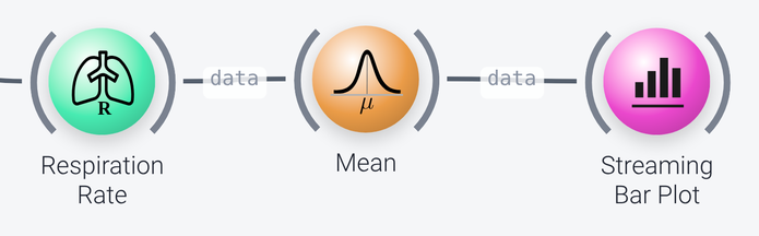
The Respiration Rate node estimates the respiration rate in breaths per minute, from the detected R peaks. It works on a sliding window that is 60 seconds long (window_length) and that is moved by 1 second on every update (window_shift). The minimum_respiration_rate and maximum_respiration_rate properties (10 and 28 breaths per minute here) set the range of rates that is considered, and smooth_it is enabled to smooth the result. As for the other measures, a Mean node averages the output along the time axis, and the result is shown on a Streaming Bar Plot (y_limits of 0 to 30).

Plotting the ECG Signal

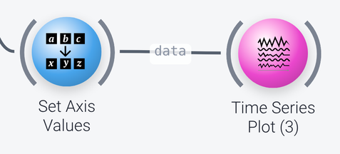
The R Detection node also passes on the ECG signal, and a Time Series Plot shows it together with the detected peaks, which are indicated by vertical lines. Since the Mean node renamed the channel to average, a Set Axis Values node first renames it to ECG for the plot. The plot shows the last 5 seconds of the signal (time_range).

The vertical lines come from the event markers in the data that R Detection sends out. Its output packet contains two streams: the ECG signal and, in addition, a stream with the times of the detected R peaks, whose name is that of the signal stream with -peaks appended. This second stream is a stream of events (the peak times are in its instance axis). The whole packet is wired into the Time Series Plot, which plots the signal stream (since its stream and stream_name properties are not set, it plots the first signal stream in the packet), and, since its plot_markers property is enabled, it also draws every event of the marker stream as a vertical line at its time, in the color set by the marker_color property (here red). If you disable plot_markers, only the ECG signal is shown.