Connectivity Estimation

The connectivity estimation pipeline example demonstrates how NeuroPype can be used to extract brain source activity from multiple brain regions, and how these activity estimates can be used to estimate directed information flow between brain regions using granger causal approaches in real time.

The main pathway of the pipeline is shown in the following figure:

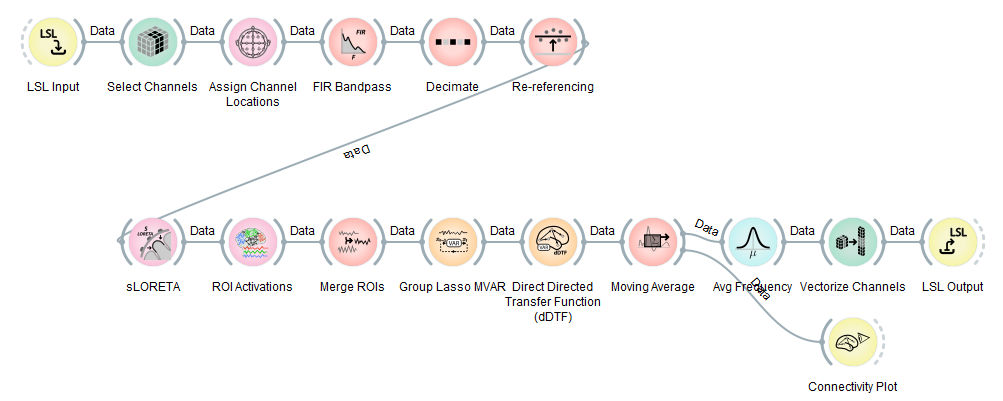
The processing done by this pipeline can be divided into multiple stages, including EEG data acquisition, pre-processing, source activity estimation, connectivity modeling, post-processing, and output.

Data Acquisition

For data acquisition we use the lab streaming layer (LSL) like in the other example pipelines. The input node is set up to read from a particular named data stream, which happens to be the one that is provided by the three nodes at the bottom of the pipeline, which play back a recording of EEG data over LSL, shown below:

To switch the input over to a live EEG device, we recommend removing the three playback nodes, and changing the LSL Input node's Query parameter from a name-based query to one that basically causes it to read from any EEG stream, using the string type='EEG'. Alternatively, you can also use a name-based query as before, but use the name of the actual live EEG LSL stream (these names can be looked up in the list of current LSL streams, which is opened up by the menu item Help/LSL Streams). You can always go back to playback by running the StreamPlaybackData example pipeline in a separate pipeline (ideally using a recording from your own EEG hardware).

Preprocessing

The pre-processing pathway, shown below, is similar to that of other source localization pipelines, and for completeness we repeat it here.

First, we retain the subset of data channels that contain EEG, since non-EEG channels, such as trigger, accelerometer, ExG, etc., will throw off the source localization stage. The Select Channels node is currently set up to remove the last 5 channels of the data, which here happen to be such miscellaneous channels. Note the tooltip for this parameter, which explains the various syntax options in more detail.

Next, we need to associate each channel with a location on the scalp, since otherwise we would have no frame of reference to estimate brain source activity from. If your channels are in the international 10-20 system (or the finer-grained 10-5 system), this step will work out of the box, but if you have other kinds of montages, you may need a custom montage file. See documentation of this node for more information on this.

In the next step, we remove unwanted frequency components from the EEG using a 1-45Hz bandpass filter. This filter will remove both slow drifts, as well as high-frequency activity such as power line noise from the data. The specific frequency response of this filter could be tuned somewhat to better match a specific application.

The next node in this setup is performing a resampling, which here is set to reduce the sampling rate by half. As explained further in the documentation of this node, the node requires that the input signal contains no frequency contents above 1/2 of the new sampling rate (the Nyquist frequency), since otherwise spectral aliases would appear -- this is the second function of the FIR filter, which happens to remove these high frequencies together with other unwanted frequencies. The main purpose of this resampling is to increase the processing speed of the pipeline so that it runs well on slower machines. If you have plenty of CPU power or speed is a lesser concern for you, you can drop the decimation without a second thought (though if your EEG system provides very high sampling rates such as 2 or more KHz, you probably should keep the decimation in).

Lastly, we change the reference of the data using the re-referencing node. Specifically, we change to a common average reference, that is, we remove the average of all channels from each channel. This step is crucial when using source localization features of NeuroPype, since NeuroPype's head models assume that the data has been common-average referenced.

Source Estimation

The next steps compute the source activity across the brain and then compute average activity in specific select brain regions, shown below:

In the first step, we calculate the activity for each source location in the brain, which is, when using the NeuroPype default head model, the set of vertices of a mesh that follows the contours of the brain (based on the Colin27 brain). It is possible to use one of several alternative nodes here, such as sLORETA, eLORETA, or LCMV Beamforming. For this example, we use sLORETA. This node has one main option, namely the head model to use. The NeuroPype Suite ships with a standard head model. There is also a tunable parameter that can be used to adjust the smoothness of the source reconstruction. Further, there is an experimental feature that allows to adapt the headmodel to channel labels and locations that are not in the 10-20 system, using the interpolate checkbox. If this applies to you, be sure to read the parameter's documentation before you use it. The output of this node is a time series with one channel for each vertex (of which there are over 4000).

Next, we want to compute the average activity of a few entire brain regions rather than thousands of small patches of cortex, among others to reduce dimensionality and make it more tractable to compute information flow between these regions. To this end, we first compute the average activity in pre-defined regions of interests (ROIs). These regions form a parcellation of the brain surface into specific named anatomical regions, and they are pre-defined by what is called a brain atlas. A head model file may contain one or more atlases, in this case it contains one (the Desikan-Killiany atlas with 467 regions). Unless we want to use a non-standard atlas or only a subset of the regions, we can use the default settings of the ROIActivations node for this, which will output a time series with one channel for each region. To learn where each of the regions is located, have a look at the companion article for the D-K atlas.

Last, we intend to compute the average activity time course for a small subset of regions, which also happen to be larger than the parcels defined in the atlas. So the goal is to compute a time series with fewer channels, each of which has the average activity of a specific group of atlas regions, that is the average of a specific subset of input channels. If we had only one or a handful of target regions, we could use the Select ROIs node to make a selection and then the Mean node to average the result into a channel, and do this process for each of our target ROIs -- however, since we have quite a few target regions, the amount of repetitive wiring in the pipeline would be rather cumbersome, and so we use a special-purpose node called Merge ROIs, which can merge down multiple sets of ROIs into a new set of target ROIs. The description of what shall be merged and how it should be called is written as a textual description, using a bracket syntax that should be familiar to Python users -- you can find an explanation and some examples in the node's documentation. When editing this, it helps to copy-paste the content of the parameter edit field into a text editor and possibly line-break the text to get a good grasp of what is merged into what, and to carefully review that all desired regions are included. The list of regions that are available for use can also be found in a file named the same as the head model, but ending in -atlas-labels.txt, under NeuroPype Enterprise/resources/headmodels.

Connectivity Modeling

The connectivity modeling is here done in two stages, using the below two NeuroPype nodes:

The approach used here first estimates a (time-varying) multivariate autoregressive (MVAR) model that describes the dynamics of the system (the select set of regions), and then we estimate directed information flow between the involved regions from this MVAR model. The Group Lasso MVAR node is a powerful approach for MVAR modeling, which is also fast enough for real-time use as long as there are not too many regions or excessively high sampling rates or model orders involved. The main assumption used by this node to make the inverse modeling problem statistically tractable is that at a given time likely not every region strongly drives the activity in each other region, but that the connectivity is "sparse", that is, only a subset of connections between regions are active. The node is quite robust to a variety of data, but when applying the setup to a different set of regions or EEG system it is recommended to make sure that the parameters are reasonably well-chosen. One simple way to this end is to review the output and make sure that the estimated connectivity is not pathological, that is, either no connectivity at all (too sparse), or everything is connected with everything else (non-sparse solution). The main parameter to adjust to ensure that the node operates in a healthy regime is the degree of sparsity (also known as regularization strength). To a lesser extent there are several parameters that determine the complexity of the model (model order), the amount of data available for estimation (window length), parameters that guide the fitting procedure (rho, alpha), and parameters that serve as the stopping criterion (max iterations, tolerance). These parameters can be adjusted to ensure the algorithm runs in a healthy regime -- see documentation for each parameter. These settings also trade off the running time and the accuracy of the resulting solution.

Once we have the MVAR model, the next step is straightforward. Essentially, we can use any of a number of alternative dynamical measures (see nodes in the connectivity category) to describe the system dynamics, including, for instance, partial directed coherence or direct directed transfer function. One of the highest-quality measures is the standardized directed transfer function (sdDTF), which is the one used in this patch following the MVAR modeling. The output of this node is for every time step and every frequency a square matrix that describes the degree of information flow from a given source (here: region) to any other source. When NeuroPype processes a new chunk of EEG, the output of this node is a 4-way tensor, indexed by (time, frequency, region, region), which describes this interaction as it changes over time.

Postprocessing and Output

The connectivity solution is quite a rich representation, and can be used for a variety of purposes. Here, we prepare the results for visualization by smoothing over time (yielding a more slowly changing estimate), and by averaging over all frequencies of interest. Then we are ready to plot the connectivity using the Connectivity Plot node, and also to send the data out over LSL. Since LSL only supports a flat list of channels, we also need to vectorize the regions by regions matrix before we send it off.

Copyright (c) Syntrogi Inc. dba Intheon. All Rights Reserved.