Spectral power in regions of interest

This example pipeline, ROISpectralBandPowerEstimation.pyp, estimates the spectral power in selected brain regions of interest (ROIs) from a live EEG stream. The EEG is preprocessed, the activity of the brain sources is estimated with sLORETA, and the activity is averaged over the selected regions. For these, the power spectrum is computed in a moving window, and it is plotted, as well as the average band power in the standard frequency bands.

The first part of the pipeline, up to the source estimation, is also used in the connectivity estimation example. The source estimation can be done with sLORETA, as in this pipeline, or with a beamformer, as described in the section on source estimation.

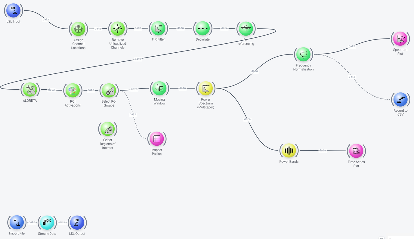
The pipeline can be divided into five parts, which we discuss in the following: data acquisition and preprocessing, source estimation and region selection, spectrum computation, normalization and plotting, and band power.

Data Acquisition and Preprocessing

Includes: LSL Input, Assign Channel Locations, Remove Unlocalized Channels, FIR Filter, Decimate and Re-referencing

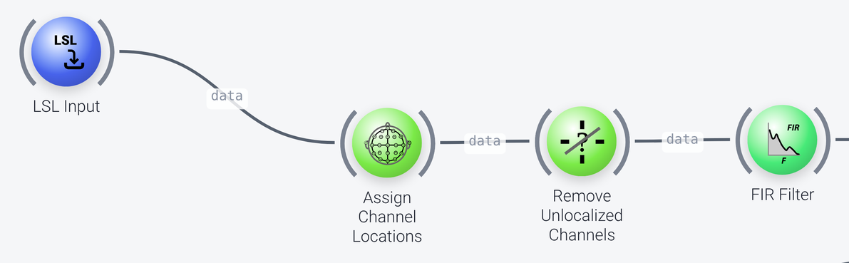
The pipeline receives its EEG data from the lab streaming layer through the LSL Input node, whose query property is set to name='MyOutputStream'. The three nodes at the bottom of the pipeline (Import File, Stream Data and LSL Output, which are not shown in the screenshots) play back a recording, VisualArrest.xdf, over LSL under that name, so that the example can be run without a live data source. For use with live data, remove them and change the query property of LSL Input so that it finds the stream of your device. See Data input in the example pipelines for more on this setup.

The preprocessing nodes are:

• Assign Channel Locations and Remove Unlocalized Channels: devices often send out non-EEG channels. These two nodes assign each channel a 3D location based on standard montages, and then remove the channels that are not found in a montage (i.e., the non-EEG channels). This is important to not mess up the downstream nodes, in particular the source estimation.
• The FIR Filter is a band-pass filter (frequencies of 0.5, 1, 45 and 50 Hz), so no frequencies outside of 1 to 45 Hz will be seen in the results.

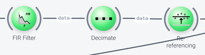
• Decimate is a very fast way of downsampling the data (here by a factor of 2), for performance reasons. Note that this node does not use an anti-aliasing filter, which is why it follows the low-pass of the FIR Filter.
• Re-referencing is set up to do common average referencing (its reference_range is :, all channels). Depending on your device, you may instead specify the reference channels here. The source estimation requires that the data is common-average referenced.

Source Estimation and Region Selection

Includes: sLORETA, ROI Activations, Select ROI Groups and Select Regions of Interest

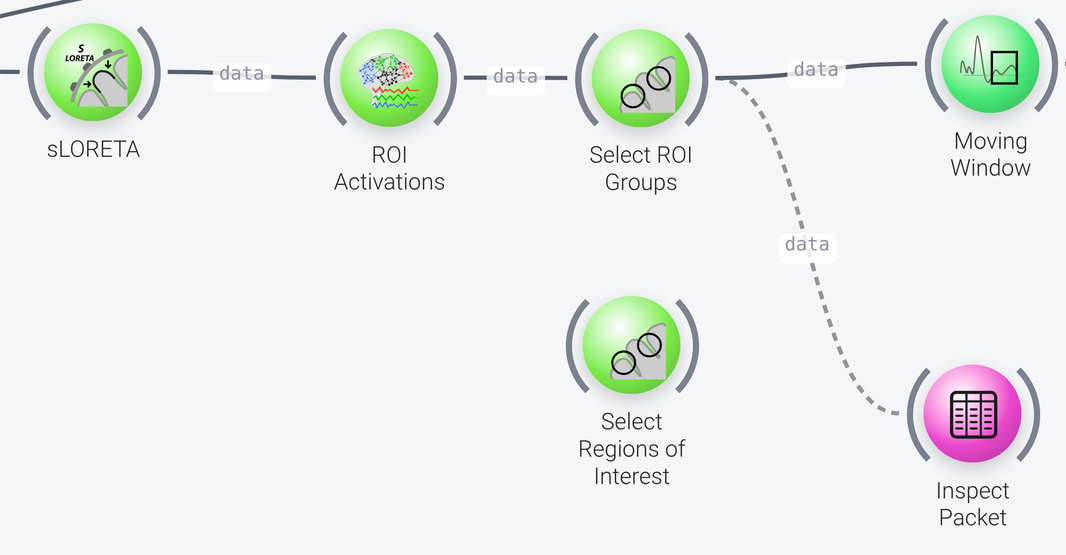
The sLORETA node estimates the brain source activity (the current source density) from the EEG, for each source location of the head model. Its properties are:

• headmodel sets the head model. Here it is a standard model based on the Colin27 brain (Colin-339ch-4495v-scalar-4shell-1.1.hm), which ships with NeuroPype, and whose source locations are the over 4000 vertices of a mesh that follows the brain surface. If you have a custom head model, you can specify it here (see the documentation of the node).
• regu is the regularization strength (0.05 here). Larger values give smoother source reconstructions.
• interpolate is for EEG systems whose channel labels are not in the international 10-20 system (or its finer-grained 10-5 variant), which is what the head model is matched against by default. If this applies to you, you can enable it to match the head model by the channel locations instead (which must be known, and in the same coordinate system as the default 10-5 locations). Read the documentation of the property before using it.

Using a beamformer instead of sLORETA

The sLORETA node can be replaced by an LCMV Beamforming node, which estimates the source activity with a linearly constrained minimum variance (LCMV) beamformer. It makes different assumptions than sLORETA. It can give a more accurate reconstruction of the sources of interest in the presence of noise, but a less focal one for a single, well-isolated source. The nodes that follow work the same way, since the output is again a time series with one channel per source location.

The beamformer has two inputs: data, which receives the common-average referenced EEG just like sLORETA, and covariance, which receives a running estimate of the covariance of the data. This can be computed from the re-referenced EEG by a Per-Element Covariance node, followed by an Exponential Moving Average node (or a Moving Average node) that smooths it over time. Read the documentation of the averaging node to understand what time range is used for the estimate. (When processing recorded data, it is recommended to segment the data first.) The headmodel and interpolate properties are the same as in sLORETA. The shrinkage property (0.001 by default) regularizes the covariance matrix, which can become degenerate when the window is short or there are many channels, and the default is usually fine.

The ROI Activations node then computes the average activity in the regions of interest that are defined in a brain atlas (by default the Desikan-Killiany atlas), which gives a time series with one channel for each region. Select ROI Groups selects among the major groups of regions of this atlas, here the group lateraloccipital (its selection property).

The Select Regions of Interest node is an alternative to Select ROI Groups (it is not wired up in this pipeline), which allows a more fine-grained selection of individual ROIs, such as lateraloccipital L.1. This node is designed for the Desikan-Killiany atlas. If you select a different atlas in the ROI Activations node, you need to use a Select Range node instead of this one, to list the names of the ROIs (the "channels" of the space axis) that you want to select.

The Inspect Packet node is connected to Select ROI Groups by a disabled (dashed) wire. You can enable it, by right-clicking the connecting wire and selecting Enabled, to see the list of the selected ROIs.

Spectrum Computation

Includes: Moving Window and Power Spectrum (Multitaper)

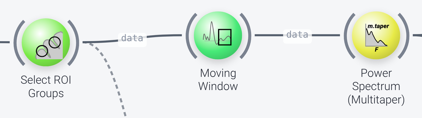
A spectrum is computed over windows of data, not over continuous data. The Moving Window node therefore outputs the most recent window of 5 seconds (window_length) on every update, and the Power Spectrum (Multitaper) node computes its spectrum. The data now has a frequency axis. The multitaper method averages the spectrum over multiple tapered windows, and the spectrum can be smoothed by increasing its half_bandwidth property. You could use the Power Spectrum (Welch) node instead.

Normalization and Plotting

Includes: Frequency Normalization, Spectrum Plot and Record to CSV

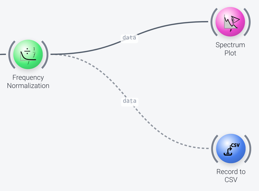
The Frequency Normalization node corrects the spectrum for the 1/f fall-off that is typical of EEG power (its alpha property, the exponent, is 1). The result is shown on a Spectrum Plot, with a title of Spectral Power for selected ROIs, and an x_range of 0 to 50 Hz, since we do not want to plot frequencies above that. Note that the Spectrum Plot also has an option to do the 1/f correction itself (one_over_f_correction), so if you enable it, you can drop the Frequency Normalization node.

The dashed wire to the Record to CSV node is disabled. If you enable it (right-click the wire), the values are recorded to a CSV file (the filename property, roi_spectral_power.csv). You could do the same for the band power values below.

Band Power

Includes: Power Bands and Time Series Plot

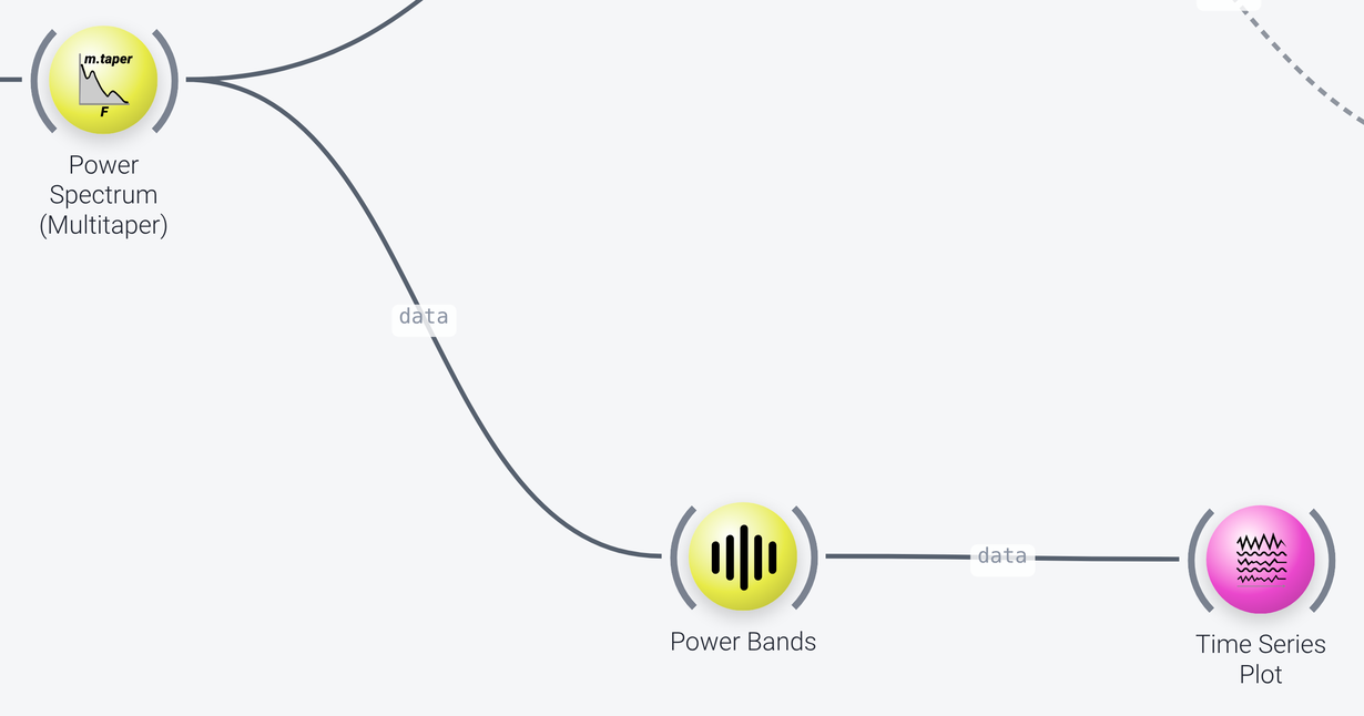
The Power Bands node takes the computed spectrum and averages it into the five standard bands (delta, theta, alpha, beta and gamma, with the default ranges of the node, which you can change with the properties of the same names), applies the 1/f correction (correct_for_falloff) and converts the values to dB (unit). The result has a feature axis with five items (the bands), instead of a frequency axis, and average_across_channels is enabled, so that the values are averaged over the selected regions. See the band power example for more on this node. A Time Series Plot shows the result over time (the last 30 seconds, time_range), with the time and feature axes plotted (its y_axis is feature).