ERP analysis of a flanker task (offline data)

This example pipeline, ERPanalysisFlankerOfflineData.pyp, analyzes the event-related potentials (ERPs) of a recording of a flanker task, comparing the trials on which the participant responded correctly with those on which the response was incorrect. It imports and preprocesses the recording, curates the event markers, computes the average ERP for each condition, plots the ERP waveforms, and finds and plots the amplitude and latency of the P300 peak. The results are also saved to CSV files.

This pipeline processes recorded ("offline") data, not a live data stream. In a pipeline that processes offline data, each node is executed once, and the entire data set is passed from one node to the next. The pipeline stops when all nodes have finished processing the data. This is unlike a streaming (online) pipeline, which receives a few samples at a time from a device or another application, and passes them through the pipeline, so all nodes are executed for each batch of samples received. The pipeline continues running indefinitely until it is stopped (if no more data comes through, the pipeline will continue to run but do nothing). See the tutorial on streaming vs. offline data for more on this.

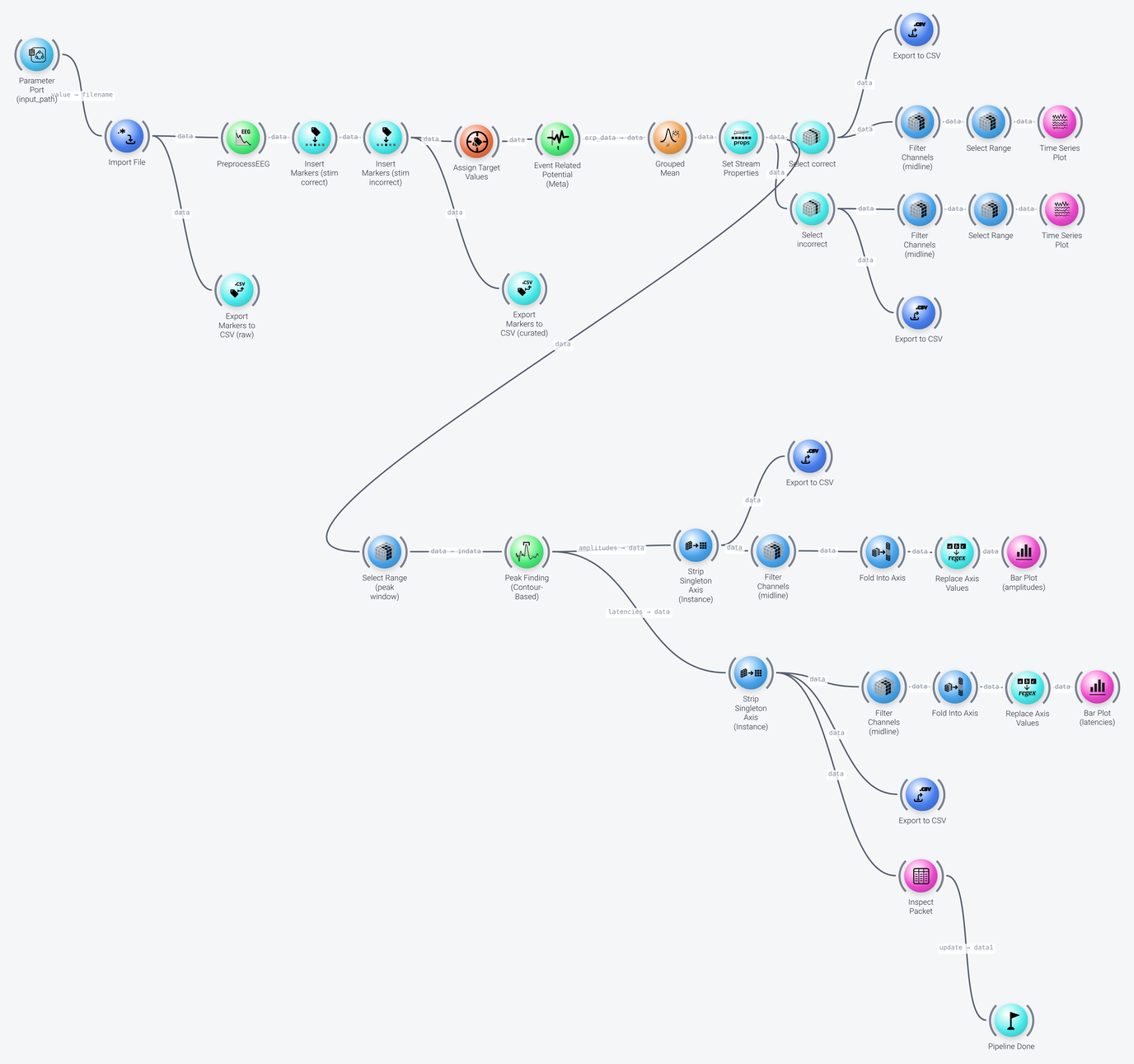
The pipeline can be divided into five parts, which we discuss in the following: import and preprocessing, marker curation and ERP calculation, plotting the waveforms, finding the peaks, and plotting and exporting the peaks. The files that the pipeline writes are listed in the last section.

Import and Preprocessing

Includes: Parameter Port, Import File, PreprocessEEG and Export Markers

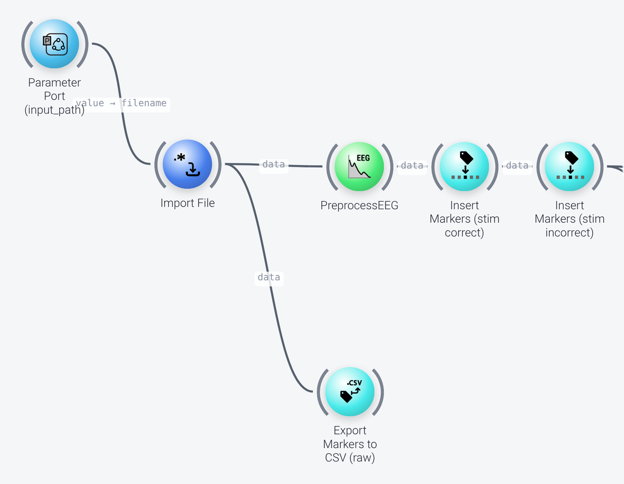
The recording is loaded by the Import File node. Its file name comes from the Parameter Port named input_path, whose default is the example file FlankerTest.set, so that the file can be chosen when the pipeline is launched. The raw markers can be exported for validation by the Export Markers node (named Export Markers to CSV (raw)), which writes the markers and their time stamps to a CSV file.

The PreprocessEEG node is a "meta-node" (a node which calls a sequence of other nodes) that performs the entire standard EEG preprocessing chain for offline data, calling a number of other nodes in order: fixing the unit of the signal, assigning channel locations, filtering, bad channel and artifact removal, interpolation of the removed channels, re-referencing and removal of bad time windows (see the documentation of the node for the full list). Here, it is set up with a low-pass filter at 30 Hz (lowpass_frequencies of 30 and 35 Hz) to reduce high-frequency noise, a high-pass filter at 0.1 Hz (highpass_frequencies of 0.1 and 0.5 Hz), and a notch filter for the line noise at 60 Hz (notch_frequency). Compare the Artifact removal example, which uses the individual nodes of the chain.

Marker Curation and ERP Calculation

Includes: Insert Markers, Assign Target Values, Event Related Potential (Meta) and Grouped Mean

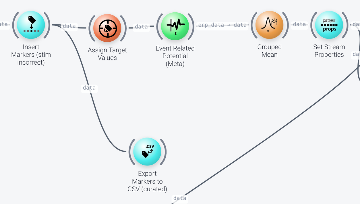
The recording contains markers for the stimuli and for the response feedback, correct or incorrect. To compute ERPs for the two kinds of trials, new stimulus onset events that are labeled with the correct or incorrect response of the trial are first inserted, using the response feedback markers. This is done by two Insert Markers nodes, one for each condition. Each of them inserts a new marker (its payload, here stim-correct or stim-incorrect) for each stimulus marker (the anchor_marker, here matching 'S' in Marker) that is followed by the corresponding response marker (the second anchor marker, anchor_marker_B, Marker=='correct' or Marker=='incorrect'). You would need to adapt these to the markers in your data, of course.

The curated markers are exported by the second Export Markers node, for validation.

Assign Target Values then selects the markers that the segments are cut around, stim-correct and stim-incorrect (the mapping property).

The Event Related Potential (Meta) node is another meta-node that segments the data around the markers that were assigned as targets, and calculates the ERPs. Here, the segments go from 0.3 seconds before to 1 second after the stimulus (time_bounds of -0.3 and 1), where 0 is the stimulus onset, and the baseline, the average from -0.3 to 0 seconds (baseline_removal_range), is removed from each trial. The output_measure property is trials, and the average ERPs are sent out through the erp_data port of the node (the other output, not used here, is an ERP image, which is not averaged across all trials).

The Grouped Mean node averages the trials by condition, i.e., the Marker (its group_cols property), which gives the average waveform of the stim-correct and of the stim-incorrect trials. The Set Stream Properties node then sets the stream property has_markers to False.

Plotting the Waveforms

Includes: Select Instances, Select Range and Time Series Plot, and Export to CSV

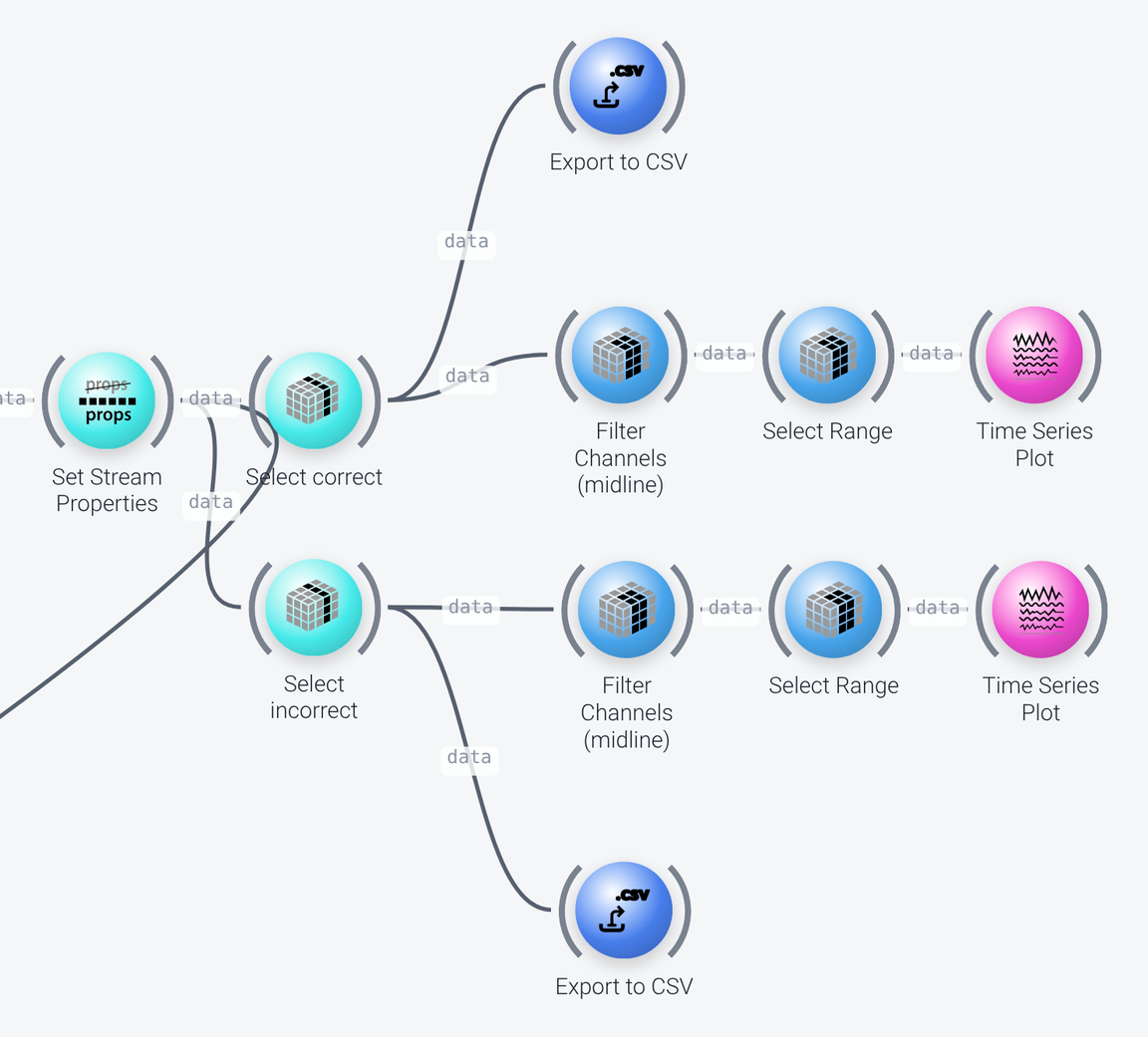
Two Select Instances nodes (named Select correct and Select incorrect) split the averaged waveforms into the two conditions, by keeping the instances whose Marker is stim-correct or stim-incorrect (the selection property). The waveforms of each condition are then plotted and saved:

• An Export to CSV node saves the mean waveforms of all the channels to a CSV file, with one row per channel (row_axis of space) and one column per time point (col_axis of time).
• For the plots, a Select Range node (named Filter Channels (midline)) first selects the midline channels Fz, Cz and Pz. A second Select Range node keeps the first 0.5 seconds (0...0.5 on the time axis), and a Time Series Plot shows the result.

Note that if you want to save the ERPs for all the channels, the export node needs to be placed before the node that selects the midline channels, as it is here.

Finding the Peaks

Includes: Select Range, Peak Finding (Contour-Based) and Strip Singleton Axis

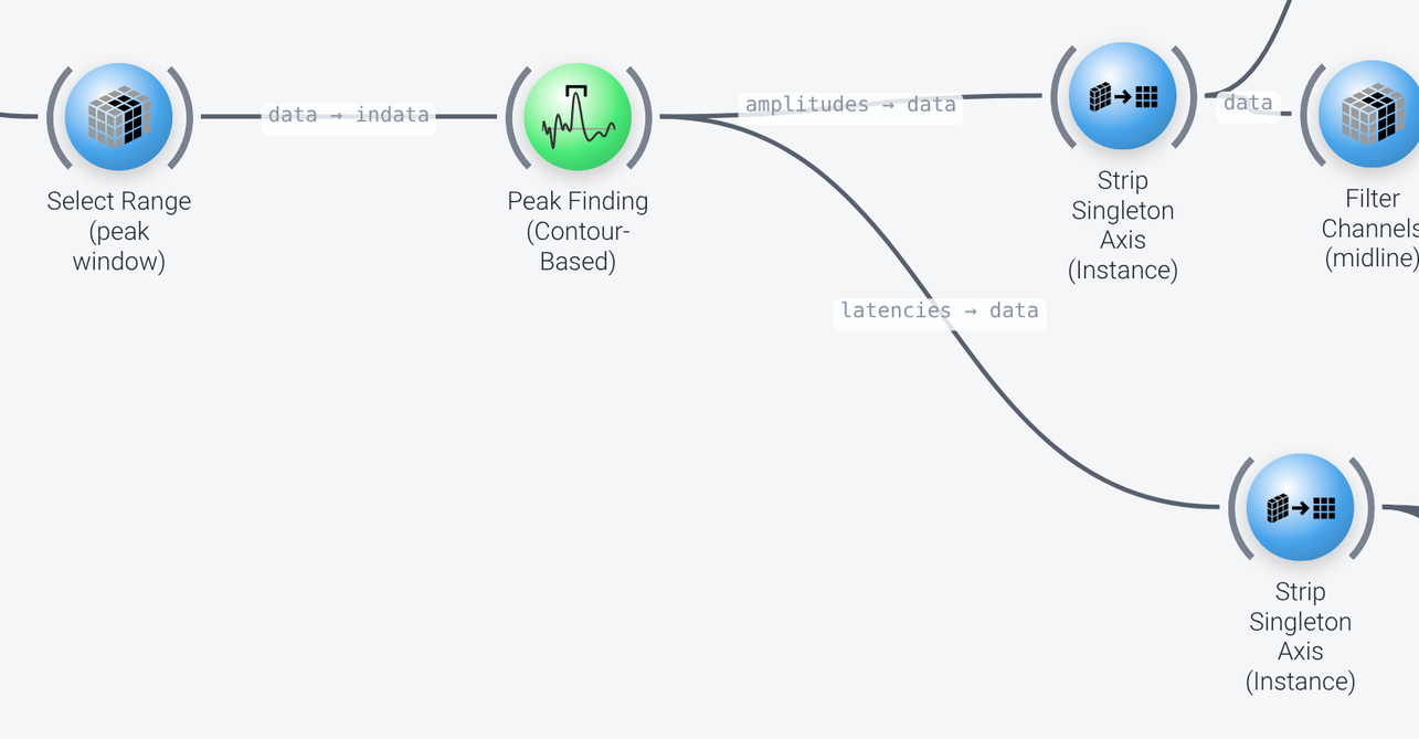
The second part of the pipeline finds the amplitude and the latency of the P300 peak of the ERP. It takes the averaged waveforms from the Set Stream Properties node (see the screenshot in the previous section), and a Select Range node (named Select Range (peak window)) keeps the time window in which the peak is expected, 0.2 to 0.5 seconds (0.2...0.5 on the time axis).

The Peak Finding (Contour-Based) node finds the peaks in the data along the time axis (axis property). With max_count set to 1, it finds only the highest peak in each waveform, and it reports the position of the peak in seconds (unit, and account_for_time_axis). It has two outputs, the amplitudes and the latencies of the peaks, and each of them goes to a separate branch: it is important to connect the desired output port in nodes that have multiple output options.

The peak finding node adds a second, singleton instance axis for each peak component, with the label peaks. A Strip Singleton Axis node removes this extra axis, for plotting and export, by referencing it by its type and label (axis of instance.peaks).

Peak Amplitudes

Includes: Strip Singleton Axis, Export to CSV, Select Range, Fold Into Axis, Replace Axis Values and Bar Plot

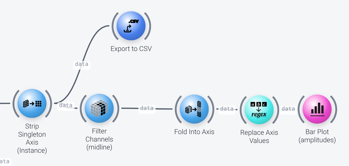
The amplitudes are saved to a CSV file by an Export to CSV node, with one row per channel and one column per instance (col_axis property set to instance, which represents the trials), and are plotted on a bar plot, for the midline channels only.

For the plot, the data is reduced to one dimension: a Select Range node (Filter Channels (midline)) selects the channels Fz, Cz and Pz, and a Fold Into Axis node combines the channels (the space axis) with the instances (the instance axis, folded by Marker), so that the names of the resulting elements have the form channel-condition. The names are then cleaned up by a Replace Axis Values node, which removes the word stim and other details of the instances (the target assignment, the trial numbers and totals) using a regular expression (pattern_type of regex), and the result is shown on a Bar Plot titled Midline Channels Peak Amplitudes (uV).

Peak Latencies, and Finishing the Pipeline

Includes: Strip Singleton Axis, Select Range, Fold Into Axis, Replace Axis Values, Bar Plot, Export to CSV, Inspect Packet and Pipeline Done

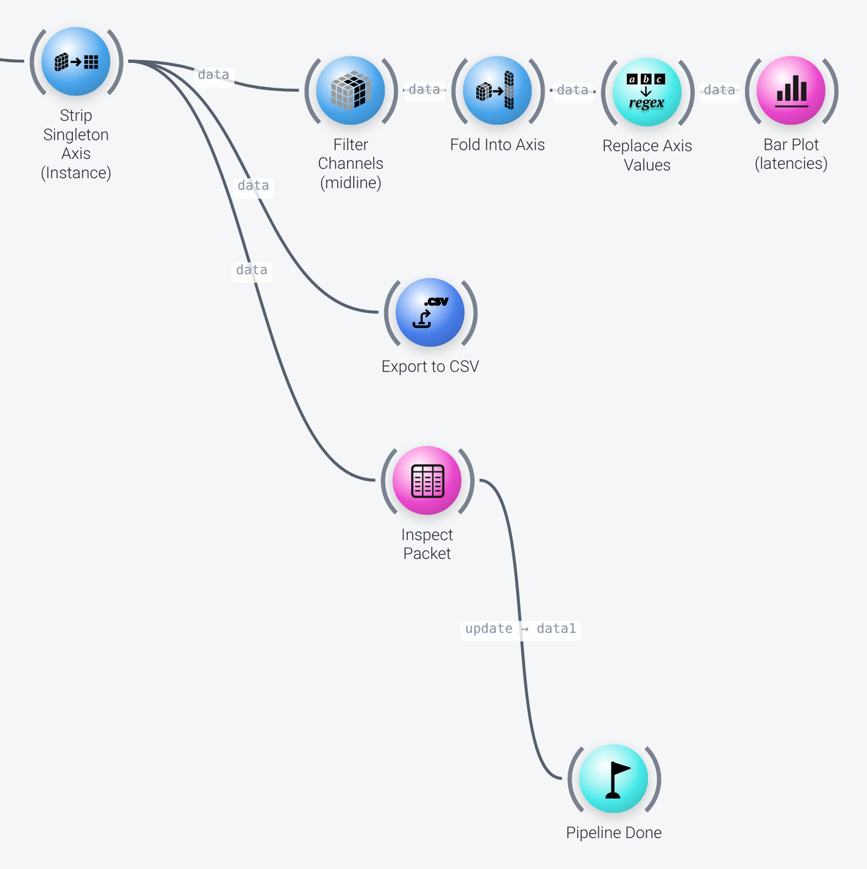
The latencies are processed in the same way as the amplitudes: they are plotted on a Bar Plot for the midline channels (with y_limits of 0.2 to 0.3 seconds) and saved to a CSV file by an Export to CSV node.

An Inspect Packet node (shown here with the title Peak Latency) displays the data and the axes of the packet in a table. Its row_axis and col_axis properties select the instance and space axes, so that the matrix that is displayed corresponds to the data that is exported to CSV.

The Pipeline Done node forces the pipeline to report that it is finished. Without it, the open plots would prevent the pipeline from being reported as finished. The update port of Inspect Packet is wired into it, since no output is expected from the Inspect Packet node, but we need to know whether it was executed (which sets its update port to True). This node is not absolutely necessary, as you can always stop the pipeline manually.

Outputs

The pipeline writes the following files (to the folder given by the output_root property of the export nodes):

• FlankerERP_raw.markers.csv: the raw markers, with time stamps
• FlankerERP_curated.markers.csv: the curated markers, with the inserted events for stimulus onset by response type
• FlankerERP_mean_correct_waveform.csv and FlankerERP_mean_incorrect_waveform.csv: the mean ERP waveforms (in µV) for the trials with correct and incorrect responses, by channel
• FlankerERP_mean_amplitudes.csv: the mean ERP P300 peak amplitudes (in µV) for correct and incorrect trials, by channel
• FlankerERP_mean_latencies.csv: the mean ERP P300 peak latencies (in seconds) for correct and incorrect trials, by channel