Spectral analysis of a recording (eyes closed vs eyes open)

This example pipeline, SpectralAnalysisVisualArrestOfflineData.pyp, computes EEG power spectra and frequency band powers for a recording of a visual arrest task, in which the participant alternates between having their eyes closed (EC) and open (EO). It imports and preprocesses the recording, cuts it into 1 second epochs for each of the two conditions, computes the power spectrum of each epoch, and averages the results by condition. The spectra and the band powers are plotted and saved to CSV files, and the difference in alpha power between the two conditions is plotted as a topography plot.

This pipeline processes recorded (offline) data, not a live data stream: each node is executed once, and the entire data set is passed from one node to the next. See the tutorial on streaming vs. offline data for more on this.

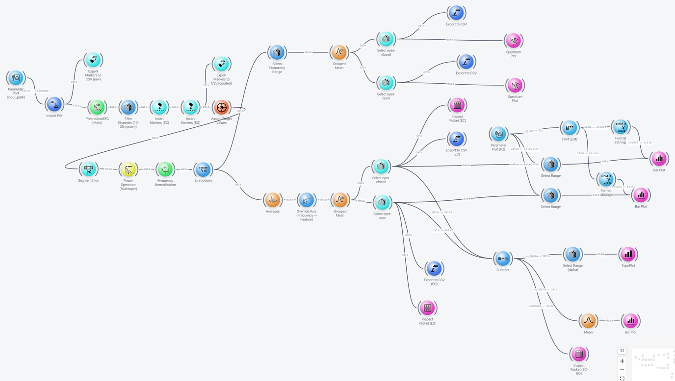
The pipeline can be divided into five parts, which we discuss in the following: import, preprocessing and marker curation; the power spectrum; spectra by condition; band powers by condition; and the difference between the conditions. The files that the pipeline writes are listed in the last section.

Import, Preprocessing and Marker Curation

Includes: Parameter Port, Import File, Export Markers, PreprocessEEG, Select Range, Insert Markers, Assign Target Values and Segmentation

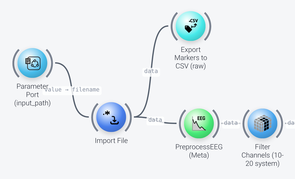
The recording is loaded by the Import File node. Its file name comes from a Parameter Port (the input_path, with the default VisualArrest.xdf), so that it can be set when the pipeline is launched. The raw markers can be exported for validation by an Export Markers node, which writes the markers and their time stamps to a CSV file.

The PreprocessEEG node is a "meta-node" that performs a whole series of preprocessing steps, which could also be run as individual nodes, as in some of the other example pipelines (for instance the artifact removal example). See the documentation of the node for the steps that it performs. Some of these steps can be skipped, depending on the parameters of the node. Here, the node is set to do a low-pass filter at 60 Hz (lowpass_frequencies of 55 and 60 Hz), so there will be no high gamma activity in the results.

A Select Range node (named Filter Channels (10-20 system)) keeps the channels of the 10-20 system that are used here.

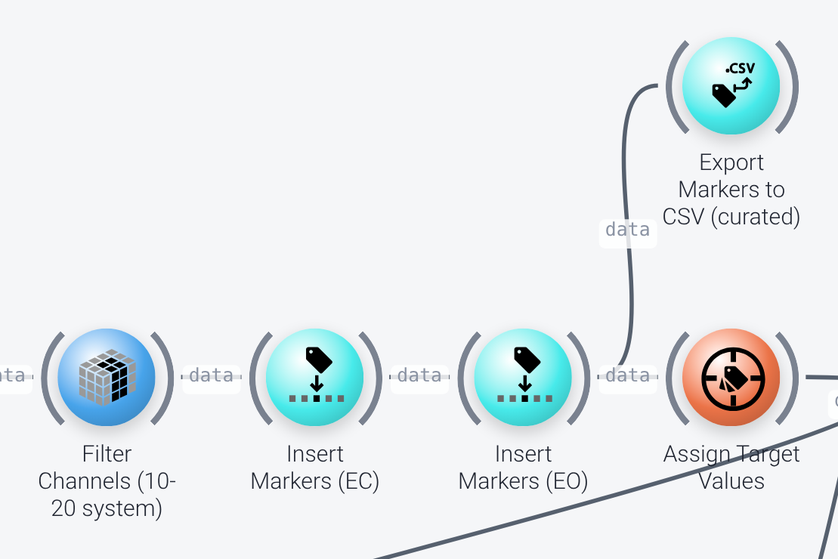
The particular recording processed here has markers for the beginning and the end of each period with eyes closed or eyes open (eyes-closed-begin, eyes-closed-end, and eyes-open-begin, eyes-open-end). To cut it into epochs, an event marker is inserted every second within each of these periods, for each of the two conditions, by two Insert Markers nodes. Each of these nodes are set to marker-locked mode and therefore act on existing event markers. They insert markers with a payload of eyes-closed or eyes-open, in the span between the begin and the end marker (the anchor_marker and the anchor_marker_B), once for every second (count of 1 and counting of persecond). The curated markers can be exported by a second Export Markers node, for validation. If the recording didn't have event markers but relied on specific timings (i.e., 30 seconds of EO followed by 30 of EC, etc.), the Insert Markers can be used in absolute or relative mode so that it acts on timestamps and not event markers.

Assign Target Values then selects these markers as the markers that the epochs are cut around (its mapping is the list eyes-closed and eyes-open), and the Segmentation node (see the next screenshot) cuts the epochs by the conditions that were assigned, from 0 to 1 second after each marker (its time_bounds).

The Power Spectrum

Includes: Segmentation, Power Spectrum (Multitaper), Frequency Normalization and To Decibels

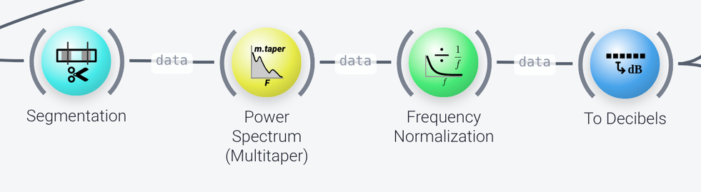
The Power Spectrum (Multitaper) node computes the power spectrum of each epoch, using the multitaper method (its half_bandwidth of 2.5 sets the smoothing of the spectrum). Frequency Normalization corrects the spectrum for the 1/f fall-off, and To Decibels converts the power values to dB. The data now has a frequency axis, and the pipeline splits into two branches, one for the spectra and one for the band powers.

Spectra by Condition

Includes: Select Range, Grouped Mean, Select Instances, Export to CSV and Spectrum Plot

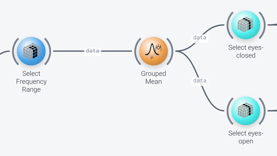
The first branch keeps the frequencies from 0.5 to 60 Hz with a Select Range node (named Select Frequency Range), and then the Grouped Mean node averages the epochs by condition, i.e., by the Marker (its group_cols property), which gives one average spectrum for the eyes-closed epochs and one for the eyes-open epochs. Two Select Instances nodes (named Select eyes-closed and Select eyes-open) split them into the two conditions, by keeping the instances whose Marker is eyes-closed or eyes-open (the selection property).

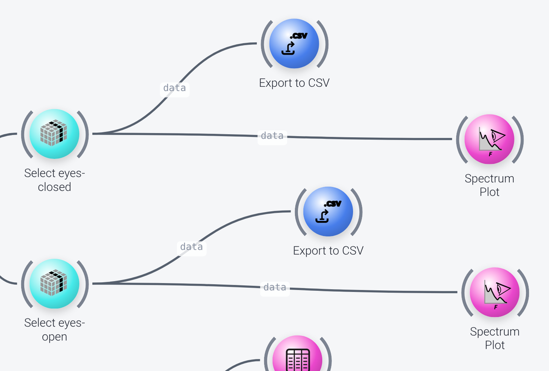
For each condition, the spectra are saved by an Export to CSV node (with one row per channel, row_axis of space, and one column per frequency, col_axis of frequency), and plotted on a Spectrum Plot (with the spectrum of each channel, stacked), whose title is Spectrum view (eyes-closed) or (eyes-open).

Band Powers by Condition

Includes: Averages, Override Axis, Grouped Mean, Select Instances, Export to CSV, Inspect Packet, Select Range, First (List), Format (String) and Bar Plot

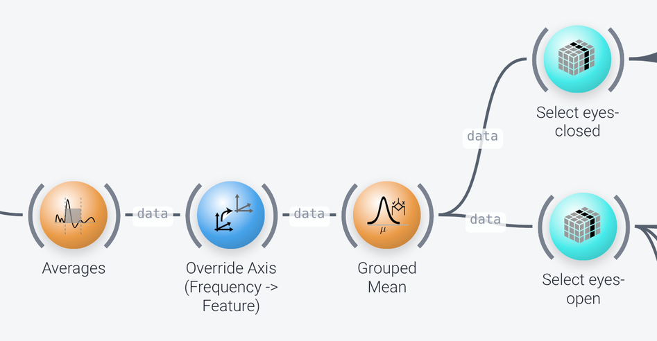
The second branch computes the band powers. The Averages node averages the frequency bins into bands, which are given by its windows property: 1 to 4 Hz, 4 to 8 Hz, 8 to 12 Hz, 12 to 30 Hz and 30 to 50 Hz. Since the data now represents bands instead of frequency bins, the Override Axis node (named Override Axis (Frequency -> Feature)) turns the frequency axis into a feature axis, so that the bands can be named: its init_data property gives the names delta, theta, alpha, beta and gamma, which appear in the exported or plotted data. As before, a Grouped Mean node averages by the condition assigned in Assign Target Values, and two Select Instances nodes select the two conditions.

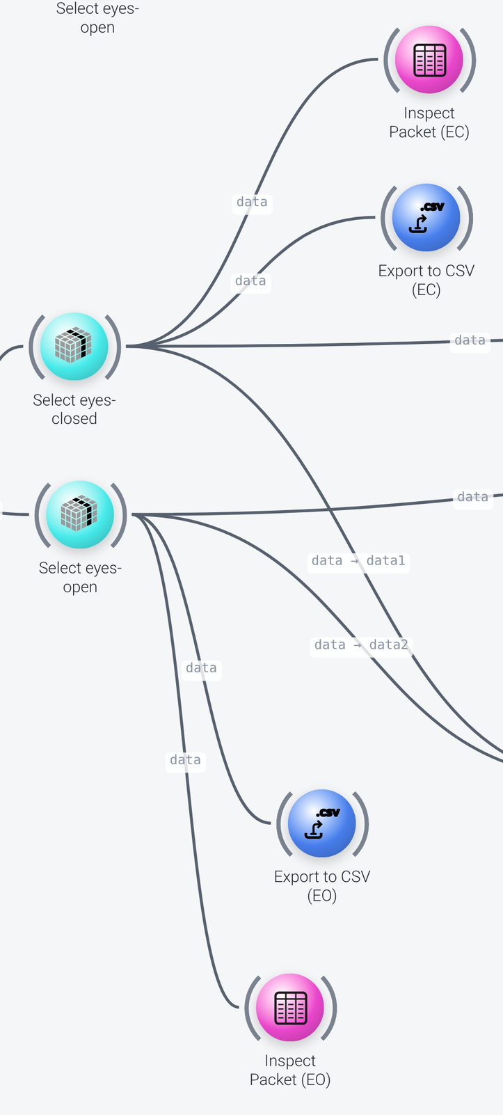
We averaged over the epochs with Grouped Mean, which reduced the data to 2 instances (one per condition), and then selected one of the two conditions, which reduces the instance axis to a single instance (item). So in terms of data, we end up with a 2D matrix of feature (the power bands) and space (the channels), which can be exported to CSV, as rows and columns, by an Export to CSV node (with a col_axis of feature). An Inspect Packet node for each condition shows this matrix (its row_axis and col_axis properties select the space and feature axes), so that you can see all the numerical band power values, by channel and by band.

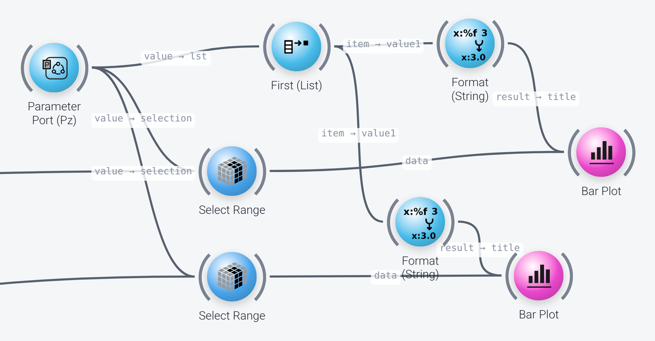
The band powers for one channel are also plotted for each condition, on a Bar Plot. The channel is chosen by a Parameter Port (plot_channel_name, default of ['Pz']) and selected by a Select Range node, since a bar plot expects a vector. As the Select Range node takes a list, a First (List) node extracts the one item of the list, so that it can be added to the plot title by a Format (String) node (for instance Band Powers (eyes-closed) [%s]), which is wired into the title of the Bar Plot.

The Difference between the Conditions

Includes: Subtract, Select Range, TopoPlot, Mean, Bar Plot and Inspect Packet

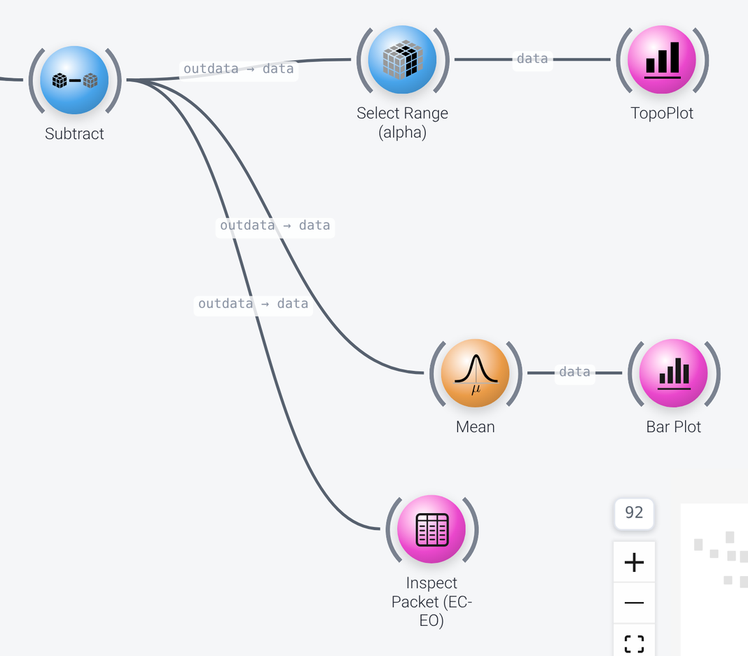
A Subtract node subtracts the band powers of the eyes-open condition from those of the eyes-closed condition. The result, the difference in power between the conditions, is used in three ways:

• A Select Range node (named Select Range (alpha)) selects the alpha band (on the feature axis, by names), and a TopoPlot (a topography plot, with a title of Alpha Power Topoplot (EC - EO)) shows the difference in alpha power on the scalp.
• A Mean node averages the difference over all the channels (axis of space), and a Bar Plot shows the difference in the band powers across all channels.
• An Inspect Packet node (EC-EO) shows the numerical values, by channel and by band.

Outputs

The pipeline writes the following files (to the folder given by the output_root property of the export nodes):

• VisualArrestSpectra_raw.markers.csv: the raw markers, with time stamps
• VisualArrestSpectra_curated.markers.csv: the curated markers, with inserted events for the 1 second epochs
• VisualArrestSpectra_spectra_EC.csv and VisualArrestSpectra_spectra_EO.csv: the mean spectral power (in dB) by frequency (in Hz), for each channel, for the eyes closed and the eyes open condition
• VisualArrestSpectra_bandpowers_EC.csv and VisualArrestSpectra_bandpowers_EO.csv: the mean frequency band powers (in dB), for each channel, for the eyes closed and the eyes open condition