Compute band power

This example pipeline, Bandpower.pyp, preprocesses and cleans an EEG stream, then computes the power in the standard frequency bands (delta, theta, alpha, beta and gamma), averaged across channels, in a moving window. The band power is plotted, and is also sent out over the network (via LSL) for pickup by another application, such as a game or a neurofeedback display. It also demonstrates a way of computing the spectral power in multiple bands at once.

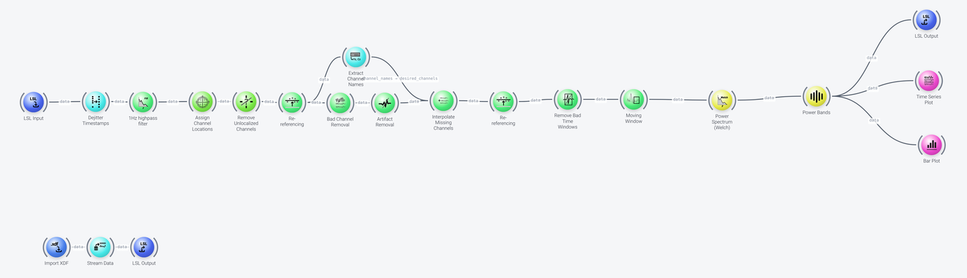
The pipeline is set up for live (streaming) data, as it is shown here, but it can also be used with offline (recorded) data, as discussed at the end of this page. It can be divided into five parts, which we discuss in the following: data acquisition, preprocessing, artifact cleaning, band power computation, and output.

Data Acquisition

Includes: LSL Input, and (for the example only) Import XDF, Stream Data and LSL Output

This pipeline is designed to run out of the box by restreaming recorded data. For use with live data, you would remove the playback branch and change the query property of the LSL Input node so that it finds your live EEG stream, for instance type='EEG', or the name of your device's LSL stream. For use with recorded data, change the Import File path, wire it directly into Dejitter Timestamps and drop the LSL and Stream Data nodes. See Data input in the example pipelines for details.

Preprocessing

Includes: Dejitter Timestamps, FIR Filter, Assign Channel Locations, Remove Unlocalized Channels and Re-referencing

The preprocessing nodes prepare the data for the cleaning nodes:

• Dejitter Timestamps makes sure that the time stamps of the incoming samples are monotonically increasing, by smoothing out their irregularities. You should generally always run this, unless the time stamps are generated by the EEG hardware itself. It is particularly necessary if the signal is acquired wirelessly (e.g., over Bluetooth), where samples tend to arrive in irregular bursts, which makes their time stamps jittery.
• The FIR Filter (named 1Hz highpass filter) is an initial high-pass filter (frequencies of 0.5 and 1 Hz) that removes slow drifts. This is required, since the Bad Channel Removal and Artifact Removal nodes assume that the data has already been high-passed. Depending on your headset and your use case, you may want to use a lower cutoff here (e.g., 0.5 Hz or even 0.1 Hz).
• Assign Channel Locations automatically assigns a position on the scalp to each EEG channel, looking up the default locations for channel labels in the international 10-20 system (or using a custom montage provided in its montage property). Downstream nodes need these locations.
• Remove Unlocalized Channels removes the channels that did not get a location, which are non-EEG channels such as triggers or accelerometers, since these have no position in a head montage.
• The first Re-referencing node, which works along the time axis, removes the mean of each channel in the time domain, i.e., any constant offset.

Artifact Cleaning

Includes: Bad Channel Removal, Artifact Removal, Extract Channel Names, Interpolate Missing Channels, Re-referencing and Remove Bad Time Windows

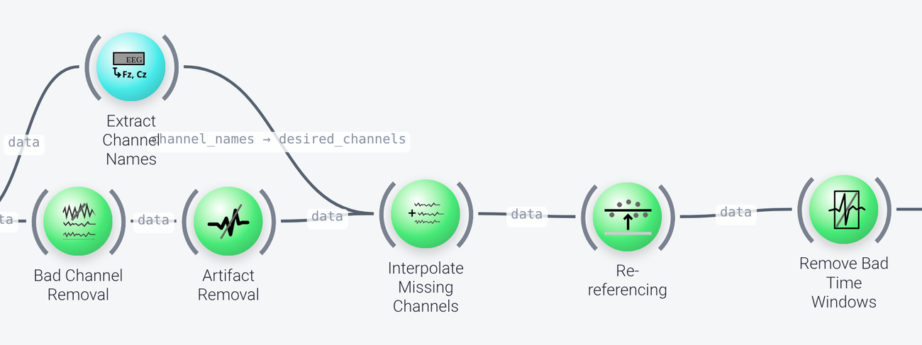
The data is then cleaned with the same chain of nodes as in the Artifact removal example, to which we refer for a detailed discussion of these nodes and of their properties. In short:

• Bad Channel Removal drops channels that are outliers (noisy or broken electrodes), and Artifact Removal removes high-amplitude artifacts such as blinks and movement artifacts using the Artifact Subspace Reconstruction (ASR) algorithm.
• Interpolate Missing Channels then restores the channels that were dropped, so that the output has the same channels as the input. The list of channels it should produce comes from the Extract Channel Names node, which reads the channel names before any channels were removed.
• The second Re-referencing node, which works along the space axis, performs common average referencing: the average of all channels (its reference_range is :) is subtracted from each channel. If you want to use a different reference, specify the reference channels in this property.
• Remove Bad Time Windows drops time segments that are still outliers after the cleaning. Note that this only works on recorded data, not live data, so this node has no effect when the pipeline is run on a live stream.

Bad Channel Removal and Artifact Removal calibrate their algorithms on the first few seconds of the stream (the calib_seconds property of each node, 30 seconds by default), so the cleaned data, and therefore the band power, only appears after this initial period.

Simplifying the preprocessing chain

For recorded data (see Using Offline Data), the nodes of the preprocessing and the artifact cleaning, from Dejitter Timestamps to Remove Bad Time Windows, can be replaced by a single PreprocessEEG node, if you prefer. It is a "meta-node" that runs a standard preprocessing chain of the same kind of nodes, in order, with their settings as its properties. This keeps a pipeline simpler, which is useful in a large pipeline. The Flanker ERP analysis example uses it. Note that PreprocessEEG only works on recorded data, not on a live stream.

Band Power Computation

Includes: Moving Window, Power Spectrum (Welch) and Power Bands

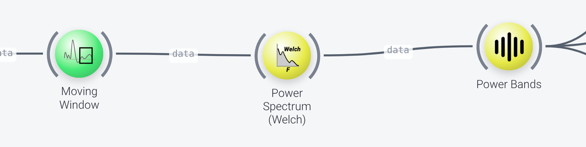
A power spectrum must be computed over windows of a certain length, not over continuous data. The Moving Window node therefore segments the stream into windows of window_length 2 seconds, and outputs the most recent window on every update. This node only works on streaming data, so it must be dropped when processing offline data (see the last section). The Power Spectrum (Welch) node then computes the power spectral density of each window.

The Power Bands node groups and averages the power spectrum into frequency bands. By default, these are the following bands (given in Hz, where the upper limit is not included):

Property	Band	Range
delta	Delta	1-3
theta	Theta	4-7
alpha	Alpha	8-15
beta	Beta	16-31
gamma	Gamma	32-40

You can change the range of each band by editing these properties, or define your own bands in the custom_bands property (for example {'theta2': [6, 7], 'beta3': [25, 31]}). If custom_bands is set, only those bands are computed, and the standard ones are ignored. Further settings used here are:

• average_across_channels is enabled, so there is only one value per band, which is the average over all channels. Disable it to get the band power for each channel separately.
• correct_for_falloff is enabled, which corrects the spectrum for the 1/f fall-off of EEG power.
• unit is set to dB, so that the band power is expressed in decibels.

Output

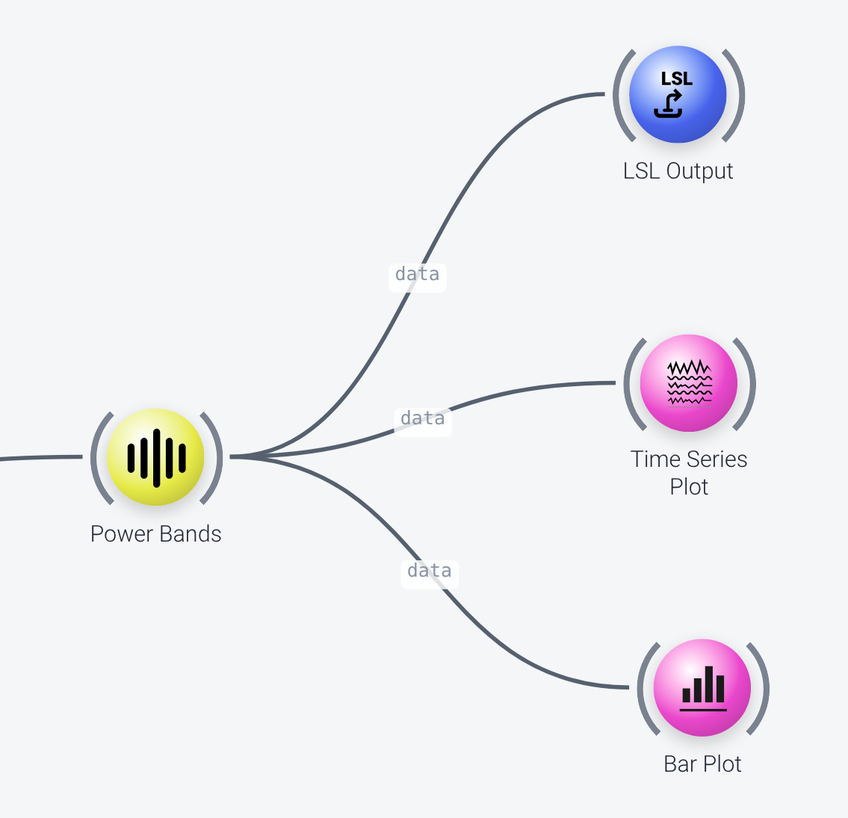
The band power is sent to three outputs:

• A Time Series Plot shows the band power over time (the last 20 seconds, its time_range property), with one line per band.
• A Bar Plot shows the current band power as one bar per band (its y_limits are 0 to 50 dB).
• An LSL Output node sends the band power out as an LSL stream named my-relaxation-1 (its stream_name property, of stream_type Control), so that it can be picked up by another pipeline or application, for example to control a game. Change the name and type to suit your application.

Using Offline Data

This pipeline can be adapted to use with offline (recorded) data. To do so:

• Wire the Import XDF node directly into Dejitter Timestamps, and drop the LSL nodes (LSL Input, and the playback branch's Stream Data and LSL Output).
• Drop the Moving Window node, since it only works on streaming data.
• Drop the LSL Output node that sends out the band power.
• The Remove Bad Time Windows node, which has no effect on live data, now becomes active.

The Bar Plot would still work and would show the average band power for the entire session, but the band power needs to be averaged over time first, which can be done by adding a Mean node (averaging along the time axis) in front of the Bar Plot.